Solution for Exercise M8.01

Solution for Exercise M8.01#

In the Chapter on Linear Models we saw that feature engineering using PolynomialFeatures can give a linear model the flexibility to capture non-linear relationships, in particular, it is useful to model interactions between features.

The downside is that the feature space grows quadratically with n_features, and if the input features are correlated, those new features would be correlated as well. Fitting a linear regressor on that many correlated features can be unnecessarily slow and prone to overfitting, even with regularization.

PCA after a polynomial expansion compresses that feature space into a smaller set of components that retain the flexibility from the non-linearly augmented feature space, before passing them to the final estimator.

In this exercise we explore whether we can tune n_components when it is used as a preprocessing step in a supervised pipeline. For such purpose we use the Ames Housing dataset, keeping only a subset of the numerical features.

import pandas as pd
import numpy as np

ames_housing = pd.read_csv("../datasets/ames_housing_no_missing.csv")
numerical_features = [
    "LotFrontage",
    "LotArea",
    "MasVnrArea",
    "BsmtFinSF1",
    "BsmtFinSF2",
    "BsmtUnfSF",
    "TotalBsmtSF",
    "1stFlrSF",
    "2ndFlrSF",
    "LowQualFinSF",
    "GrLivArea",
    "BedroomAbvGr",
    "KitchenAbvGr",
    "TotRmsAbvGrd",
    "Fireplaces",
    "GarageCars",
    "GarageArea",
    "WoodDeckSF",
    "OpenPorchSF",
    "EnclosedPorch",
    "3SsnPorch",
    "ScreenPorch",
    "MiscVal",
]
target_name = "SalePrice"
data, target = (
    ames_housing[numerical_features],
    ames_housing[target_name],
)
target /= 1000

First, fit a PolynomialFeatures with degree=2 and include_bias=False to the whole data to check how many features are produced by the polynomial expansion. You can use the attributes n_features_in_ and n_output_features_.

# solution
from sklearn.preprocessing import PolynomialFeatures

poly = PolynomialFeatures(degree=2, include_bias=False).fit(data)
print(f"Input features:                    {poly.n_features_in_}")
print(f"After degree-2 expansion:          {poly.n_output_features_}")

Input features:                    23
After degree-2 expansion:          299

With 299 features entering the ridge regressor, fit time becomes substantial. Since the original features are correlated, many of the polynomial terms are correlated as well. PCA can project them into a smaller set of uncorrelated components before fitting the predictor.

Build a pipeline with skrub.SquashingScaler using quantile_range=(5.0, 95.0), followed by the previous polynomial expansion, then PCA, and Ridge regression with default parameters as the final predictor. Use GridSearchCV with scoring set to “neg_root_mean_squared_error” to search over n_components using the grid defined below. Fit it on the full dataset.

from sklearn.decomposition import PCA
from sklearn.linear_model import Ridge
from sklearn.pipeline import make_pipeline
from sklearn.model_selection import GridSearchCV
from skrub import SquashingScaler

param_name = "pca__n_components"
param_grid = {param_name: [3, 10, 50, 100, 200, None]}

# solution
squashing = SquashingScaler(quantile_range=(5.0, 95.0))
pipeline = make_pipeline(squashing, poly, PCA(), Ridge())

grid_search = GridSearchCV(
    pipeline,
    param_grid=param_grid,
    scoring="neg_root_mean_squared_error",
)
grid_search.fit(data, target)

GridSearchCV(estimator=Pipeline(steps=[('squashingscaler',
                                        SquashingScaler(quantile_range=(5.0,
                                                                        95.0))),
                                       ('polynomialfeatures',
                                        PolynomialFeatures(include_bias=False)),
                                       ('pca', PCA()), ('ridge', Ridge())]),
             param_grid={'pca__n_components': [3, 10, 50, 100, 200, None]},
             scoring='neg_root_mean_squared_error')

In a Jupyter environment, please rerun this cell to show the HTML representation or trust the notebook.
On GitHub, the HTML representation is unable to render, please try loading this page with nbviewer.org.

Build a grid_search_results DataFrame from the attribute cv_results_ keeping only the columns listed in results_columns below.

results_columns = [
    "mean_test_score",
    "std_test_score",
    "mean_fit_time",
    "std_fit_time",
    "mean_score_time",
    "std_score_time",
    "param_" + param_name,
]

# solution
grid_search_results = pd.DataFrame(grid_search.cv_results_)[results_columns]

The following cell plots test RMSE against fit time using grid_search_results. Hover over a point to see the corresponding n_components value. It runs without modifications once grid_search_results is correctly defined.

import plotly.express as px


def plot_grid_search_results(grid_search_results):
    grid_search_results["mean_test_error"] = -grid_search_results[
        "mean_test_score"
    ]
    grid_search_results = (
        grid_search_results.drop(columns=["mean_test_score"])
        .rename(columns={"param_" + param_name: "n_components"})
        .round(2)
    )
    grid_search_results.sort_values("mean_test_error", ascending=False)

    labels = {
        "mean_fit_time": "CV fit time (s)",
        "mean_test_error": "CV score (RMSE)",
    }
    grid_search_results["n_components"] = grid_search_results[
        "n_components"
    ].fillna("None")
    fig = px.scatter(
        grid_search_results,
        x="mean_fit_time",
        y="mean_test_error",
        error_x="std_fit_time",
        error_y="std_test_score",
        hover_data=grid_search_results.columns,
        labels=labels,
    )
    fig.update_layout(
        title={
            "text": "Trade-off between fit time and mean test score",
            "y": 0.95,
            "x": 0.5,
            "xanchor": "center",
            "yanchor": "top",
        }
    )
    fig.show(renderer="notebook")

# solution
plot_grid_search_results(grid_search_results)

In general, fit times can vary significantly across runs and machines. What tends to be stable is the general shape of the curve:

The test RMSE drops substantially up to around 100 components, after which the error bars of successive points overlap. This indicates that retaining more components does not meaningfully reduce the test error.
Fit time, however, increases steadily with n_components.

The sweet spot is therefore the smallest n_components whose error bar overlaps with the best-performing point.

Does reducing dimensions stabilize the optimal `alpha`?#

During the first part of this exercise we fixed alpha to focus on the fit-time tradeoff. As we saw in the chapter on linear models, the optimal regularization strength is not necessarily the same on all cross-validation iterations. Here we ask whether reducing the number of components makes the choice of alpha more stable across folds.

Replace the Ridge from your previous pipeline to use RidgeCV(alphas=alphas). This replaces the grid search over alpha with a faster internal selection, so we only need to loop over n_components=[50, 100, None] by hand. For each component, cross_validate using ShuffleSplit (as below) and set return_estimator in the cross_validate function to collect the alpha_ attribute at each split and store them in best_alphas.

Does reducing dimensions make the optimal alpha more consistent across folds?

from collections import defaultdict

from sklearn.linear_model import RidgeCV
from sklearn.model_selection import ShuffleSplit
from sklearn.model_selection import cross_validate

alphas = np.logspace(-2, 2, 21)
best_alphas = defaultdict(list)
cv = ShuffleSplit(n_splits=50, random_state=0)

# solution
n_components_cases = [50, 100, None]
pipeline = make_pipeline(squashing, poly, PCA(), RidgeCV(alphas=alphas))

for n_components in n_components_cases:
    pipeline.set_params(pca__n_components=n_components)
    cv_results = cross_validate(
        pipeline,
        data,
        target,
        cv=cv,
        return_estimator=True,
        scoring="neg_root_mean_squared_error",
    )
    for est in cv_results["estimator"]:
        best_alphas[str(n_components)].append(est[-1].alpha_)

Make a boxplot of best_alphas using a “log” yscale.

# solution
import matplotlib.pyplot as plt

fig, ax = plt.subplots(figsize=(7, 5))
ax.boxplot(
    [best_alphas[str(k)] for k in n_components_cases],
    tick_labels=[str(k) for k in n_components_cases],
)
ax.set_yscale("log")
ax.set_xlabel("n_components")
ax.set_ylabel("Optimal alpha")
_ = ax.set_title("Stability of optimal alpha across outer folds")

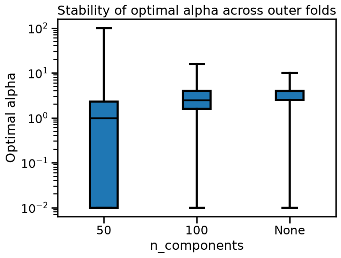
../_images/12d7864060444b141396139dcbb7343d07e7c5b7536d30d025372b95fce1ae19.png

With 50 components the interquartile range spans several orders of magnitude, while at 100 and None the distributions are compact and similar enough to each other. At 50 components the PCA representation is sensitive to which samples fall in the training fold: a different subsample changes which directions are selected, and RidgeCV compensates with a very different alpha.

Instead of changing the random_state, feel free to increase n_splits to see whether the shape of the boxes changes. Just keep in mind that increases the running time.

	estimator estimator: estimator object This is assumed to implement the scikit-learn estimator interface. Either estimator needs to provide a ``score`` function, or ``scoring`` must be passed.	Pipeline(step...e', Ridge())])
	param_grid param_grid: dict or list of dictionaries Dictionary with parameters names (`str`) as keys and lists of parameter settings to try as values, or a list of such dictionaries, in which case the grids spanned by each dictionary in the list are explored. This enables searching over any sequence of parameter settings.	{'pca__n_components': [3, 10, ...]}
	scoring scoring: str, callable, list, tuple or dict, default=None Strategy to evaluate the performance of the cross-validated model on the test set. If `scoring` represents a single score, one can use: - a single string (see :ref:`scoring_string_names`); - a callable (see :ref:`scoring_callable`) that returns a single value; - `None`, the `estimator`'s :ref:`default evaluation criterion ` is used. If `scoring` represents multiple scores, one can use: - a list or tuple of unique strings; - a callable returning a dictionary where the keys are the metric names and the values are the metric scores; - a dictionary with metric names as keys and callables as values. See :ref:`multimetric_grid_search` for an example.	'neg_root_mean_squared_error'
	n_jobs n_jobs: int, default=None Number of jobs to run in parallel. ``None`` means 1 unless in a :obj:`joblib.parallel_backend` context. ``-1`` means using all processors. See :term:`Glossary ` for more details. .. versionchanged:: v0.20 `n_jobs` default changed from 1 to None	None
	refit refit: bool, str, or callable, default=True Refit an estimator using the best found parameters on the whole dataset. For multiple metric evaluation, this needs to be a `str` denoting the scorer that would be used to find the best parameters for refitting the estimator at the end. Where there are considerations other than maximum score in choosing a best estimator, ``refit`` can be set to a function which returns the selected ``best_index_`` given ``cv_results_``. In that case, the ``best_estimator_`` and ``best_params_`` will be set according to the returned ``best_index_`` while the ``best_score_`` attribute will not be available. The refitted estimator is made available at the ``best_estimator_`` attribute and permits using ``predict`` directly on this ``GridSearchCV`` instance. Also for multiple metric evaluation, the attributes ``best_index_``, ``best_score_`` and ``best_params_`` will only be available if ``refit`` is set and all of them will be determined w.r.t this specific scorer. See ``scoring`` parameter to know more about multiple metric evaluation. See :ref:`sphx_glr_auto_examples_model_selection_plot_grid_search_digits.py` to see how to design a custom selection strategy using a callable via `refit`. See :ref:`this example ` for an example of how to use ``refit=callable`` to balance model complexity and cross-validated score. .. versionchanged:: 0.20 Support for callable added.	True
	cv cv: int, cross-validation generator or an iterable, default=None Determines the cross-validation splitting strategy. Possible inputs for cv are: - None, to use the default 5-fold cross validation, - integer, to specify the number of folds in a `(Stratified)KFold`, - :term:`CV splitter`, - An iterable yielding (train, test) splits as arrays of indices. For integer/None inputs, if the estimator is a classifier and ``y`` is either binary or multiclass, :class:`StratifiedKFold` is used. In all other cases, :class:`KFold` is used. These splitters are instantiated with `shuffle=False` so the splits will be the same across calls. Refer :ref:`User Guide ` for the various cross-validation strategies that can be used here. .. versionchanged:: 0.22 ``cv`` default value if None changed from 3-fold to 5-fold.	None
	verbose verbose: int Controls the verbosity: the higher, the more messages. - >1 : the computation time for each fold and parameter candidate is displayed; - >2 : the score is also displayed; - >3 : the fold and candidate parameter indexes are also displayed together with the starting time of the computation.	0
	pre_dispatch pre_dispatch: int, or str, default='2n_jobs' Controls the number of jobs that get dispatched during parallel execution. Reducing this number can be useful to avoid an explosion of memory consumption when more jobs get dispatched than CPUs can process. This parameter can be: - None, in which case all the jobs are immediately created and spawned. Use this for lightweight and fast-running jobs, to avoid delays due to on-demand spawning of the jobs - An int, giving the exact number of total jobs that are spawned - A str, giving an expression as a function of n_jobs, as in '2n_jobs'	'2*n_jobs'
	error_score error_score: 'raise' or numeric, default=np.nan Value to assign to the score if an error occurs in estimator fitting. If set to 'raise', the error is raised. If a numeric value is given, FitFailedWarning is raised. This parameter does not affect the refit step, which will always raise the error.	nan
	return_train_score return_train_score: bool, default=False If ``False``, the ``cv_results_`` attribute will not include training scores. Computing training scores is used to get insights on how different parameter settings impact the overfitting/underfitting trade-off. However computing the scores on the training set can be computationally expensive and is not strictly required to select the parameters that yield the best generalization performance. .. versionadded:: 0.19 .. versionchanged:: 0.21 Default value was changed from ``True`` to ``False``	False

	max_absolute_value max_absolute_value: float, default=3.0 Maximum absolute value that the transformed data can take.	3.0
	quantile_range quantile_range: tuple of float, default=(0.25, 0.75) The quantiles used to compute the scaling factor. The first value is the lower quantile and the second value is the upper quantile. The default values are the 25th and 75th percentiles, respectively. The quantiles are used to compute the scaling factor for the robust scaling step. The quantiles are computed from the finite values in the input column. If the two quantiles are equal, the scaling factor is computed from the 0th and 100th percentiles (i.e., the minimum and maximum values of the finite values in the input column).	(5.0, ...)

	degree degree: int or tuple (min_degree, max_degree), default=2 If a single int is given, it specifies the maximal degree of the polynomial features. If a tuple `(min_degree, max_degree)` is passed, then `min_degree` is the minimum and `max_degree` is the maximum polynomial degree of the generated features. Note that `min_degree=0` and `min_degree=1` are equivalent as outputting the degree zero term is determined by `include_bias`.	2
	interaction_only interaction_only: bool, default=False If `True`, only interaction features are produced: features that are products of at most `degree` distinct input features, i.e. terms with power of 2 or higher of the same input feature are excluded: - included: `x[0]`, `x[1]`, `x[0] * x[1]`, etc. - excluded: `x[0] 2`, `x[0] 2 * x[1]`, etc.	False
	include_bias include_bias: bool, default=True If `True` (default), then include a bias column, the feature in which all polynomial powers are zero (i.e. a column of ones - acts as an intercept term in a linear model).	False
	order order: {'C', 'F'}, default='C' Order of output array in the dense case. `'F'` order is faster to compute, but may slow down subsequent estimators. .. versionadded:: 0.21	'C'

	n_components n_components: int, float or 'mle', default=None Number of components to keep. if n_components is not set all components are kept:: n_components == min(n_samples, n_features) If ``n_components == 'mle'`` and ``svd_solver == 'full'``, Minka's MLE is used to guess the dimension. Use of ``n_components == 'mle'`` will interpret ``svd_solver == 'auto'`` as ``svd_solver == 'full'``. If ``0 < n_components < 1`` and ``svd_solver == 'full'``, select the number of components such that the amount of variance that needs to be explained is greater than the percentage specified by n_components. If ``svd_solver == 'arpack'``, the number of components must be strictly less than the minimum of n_features and n_samples. Hence, the None case results in:: n_components == min(n_samples, n_features) - 1	None
	copy copy: bool, default=True If False, data passed to fit are overwritten and running fit(X).transform(X) will not yield the expected results, use fit_transform(X) instead.	True
	whiten whiten: bool, default=False When True (False by default) the `components_` vectors are multiplied by the square root of n_samples and then divided by the singular values to ensure uncorrelated outputs with unit component-wise variances. Whitening will remove some information from the transformed signal (the relative variance scales of the components) but can sometime improve the predictive accuracy of the downstream estimators by making their data respect some hard-wired assumptions.	False
	svd_solver svd_solver: {'auto', 'full', 'covariance_eigh', 'arpack', 'randomized'}, default='auto' "auto" : The solver is selected by a default 'auto' policy is based on `X.shape` and `n_components`: if the input data has fewer than 1000 features and more than 10 times as many samples, then the "covariance_eigh" solver is used. Otherwise, if the input data is larger than 500x500 and the number of components to extract is lower than 80% of the smallest dimension of the data, then the more efficient "randomized" method is selected. Otherwise the exact "full" SVD is computed and optionally truncated afterwards. "full" : Run exact full SVD calling the standard LAPACK solver via `scipy.linalg.svd` and select the components by postprocessing "covariance_eigh" : Precompute the covariance matrix (on centered data), run a classical eigenvalue decomposition on the covariance matrix typically using LAPACK and select the components by postprocessing. This solver is very efficient for n_samples >> n_features and small n_features. It is, however, not tractable otherwise for large n_features (large memory footprint required to materialize the covariance matrix). Also note that compared to the "full" solver, this solver effectively doubles the condition number and is therefore less numerical stable (e.g. on input data with a large range of singular values). "arpack" : Run SVD truncated to `n_components` calling ARPACK solver via `scipy.sparse.linalg.svds`. It requires strictly `0 < n_components < min(X.shape)` "randomized" : Run randomized SVD by the method of Halko et al. .. versionadded:: 0.18.0 .. versionchanged:: 1.5 Added the 'covariance_eigh' solver.	'auto'
	tol tol: float, default=0.0 Tolerance for singular values computed by svd_solver == 'arpack'. Must be of range [0.0, infinity). .. versionadded:: 0.18.0	0.0
	iterated_power iterated_power: int or 'auto', default='auto' Number of iterations for the power method computed by svd_solver == 'randomized'. Must be of range [0, infinity). .. versionadded:: 0.18.0	'auto'
	n_oversamples n_oversamples: int, default=10 This parameter is only relevant when `svd_solver="randomized"`. It corresponds to the additional number of random vectors to sample the range of `X` so as to ensure proper conditioning. See :func:`~sklearn.utils.extmath.randomized_svd` for more details. .. versionadded:: 1.1	10
	power_iteration_normalizer power_iteration_normalizer: {'auto', 'QR', 'LU', 'none'}, default='auto' Power iteration normalizer for randomized SVD solver. Not used by ARPACK. See :func:`~sklearn.utils.extmath.randomized_svd` for more details. .. versionadded:: 1.1	'auto'
	random_state random_state: int, RandomState instance or None, default=None Used when the 'arpack' or 'randomized' solvers are used. Pass an int for reproducible results across multiple function calls. See :term:`Glossary `. .. versionadded:: 0.18.0	None

	alpha alpha: {float, ndarray of shape (n_targets,)}, default=1.0 Constant that multiplies the L2 term, controlling regularization strength. `alpha` must be a non-negative float i.e. in `[0, inf)`. When `alpha = 0`, the objective is equivalent to ordinary least squares, solved by the :class:`LinearRegression` object. For numerical reasons, using `alpha = 0` with the `Ridge` object is not advised. Instead, you should use the :class:`LinearRegression` object. If an array is passed, penalties are assumed to be specific to the targets. Hence they must correspond in number.	1.0
	fit_intercept fit_intercept: bool, default=True Whether to fit the intercept for this model. If set to false, no intercept will be used in calculations (i.e. ``X`` and ``y`` are expected to be centered).	True
	copy_X copy_X: bool, default=True If True, X will be copied; else, it may be overwritten.	True
	max_iter max_iter: int, default=None Maximum number of iterations for conjugate gradient solver. For 'sparse_cg' and 'lsqr' solvers, the default value is determined by scipy.sparse.linalg. For 'sag' solver, the default value is 1000. For 'lbfgs' solver, the default value is 15000.	None
	tol tol: float, default=1e-4 The precision of the solution (`coef_`) is determined by `tol` which specifies a different convergence criterion for each solver: - 'svd': `tol` has no impact. - 'cholesky': `tol` has no impact. - 'sparse_cg': norm of residuals smaller than `tol`. - 'lsqr': `tol` is set as atol and btol of scipy.sparse.linalg.lsqr, which control the norm of the residual vector in terms of the norms of matrix and coefficients. - 'sag' and 'saga': relative change of coef smaller than `tol`. - 'lbfgs': maximum of the absolute (projected) gradient=max\|residuals\| smaller than `tol`. .. versionchanged:: 1.2 Default value changed from 1e-3 to 1e-4 for consistency with other linear models.	0.0001
	solver solver: {'auto', 'svd', 'cholesky', 'lsqr', 'sparse_cg', 'sag', 'saga', 'lbfgs'}, default='auto' Solver to use in the computational routines: - 'auto' chooses the solver automatically based on the type of data. - 'svd' uses a Singular Value Decomposition of X to compute the Ridge coefficients. It is the most stable solver, in particular more stable for singular matrices than 'cholesky' at the cost of being slower. - 'cholesky' uses the standard :func:`scipy.linalg.solve` function to obtain a closed-form solution. - 'sparse_cg' uses the conjugate gradient solver as found in :func:`scipy.sparse.linalg.cg`. As an iterative algorithm, this solver is more appropriate than 'cholesky' for large-scale data (possibility to set `tol` and `max_iter`). - 'lsqr' uses the dedicated regularized least-squares routine :func:`scipy.sparse.linalg.lsqr`. It is the fastest and uses an iterative procedure. - 'sag' uses a Stochastic Average Gradient descent, and 'saga' uses its improved, unbiased version named SAGA. Both methods also use an iterative procedure, and are often faster than other solvers when both n_samples and n_features are large. Note that 'sag' and 'saga' fast convergence is only guaranteed on features with approximately the same scale. You can preprocess the data with a scaler from :mod:`sklearn.preprocessing`. - 'lbfgs' uses L-BFGS-B algorithm implemented in :func:`scipy.optimize.minimize`. It can be used only when `positive` is True. All solvers except 'svd' support both dense and sparse data. However, only 'lsqr', 'sag', 'sparse_cg', and 'lbfgs' support sparse input when `fit_intercept` is True. .. versionadded:: 0.17 Stochastic Average Gradient descent solver. .. versionadded:: 0.19 SAGA solver.	'auto'
	positive positive: bool, default=False When set to ``True``, forces the coefficients to be positive. Only 'lbfgs' solver is supported in this case.	False
	random_state random_state: int, RandomState instance, default=None Used when ``solver`` == 'sag' or 'saga' to shuffle the data. See :term:`Glossary ` for details. .. versionadded:: 0.17 `random_state` to support Stochastic Average Gradient.	None

Solution for Exercise M8.01

Contents

Solution for Exercise M8.01#

Does reducing dimensions stabilize the optimal alpha?#

Does reducing dimensions stabilize the optimal `alpha`?#