

Choice of n_components in the unsupervised case#
In the previous exercise we treated n_components as a hyperparameter in a
supervised pipeline. Unlike typical hyperparameters, the evaluation metric
plateaus after a certain number of components, beyond which adding more only
increases fit time. When a ground truth label is available, such plateau gives
a natural stopping criterion. When it is not, you need indirect criteria. Each
criterion encodes a different assumption about what “enough components” means,
and none of them is universally correct.
In this notebook we work through the main criteria for choosing
n_components and their implications:
Reading cumulative explained variance curves and applying 90%/95% thresholds;
using the Kaiser criterion as a threshold-free heuristic;
checking how stable both choices are under resampling;
using silhouette score to evaluate a clustering pipeline, comparing what the two criteria recommend.
We use the Wine recognition dataset throughout, pretending we do not have access to the true cultivar labels.
from sklearn.datasets import load_wine

X, _ = load_wine(return_X_y=True, as_frame=True)
The dataset contains 178 wine samples from three cultivars grown in Italy. Each sample has 13 chemical measurements, such as alcohol content, acidity, and various phenolic compounds. The goal in the original task is to identify the cultivar from the chemistry alone.
We use it here purely to practice selecting the number of PCA components on real data where the features have very different scales and units.
from skrub import TableReport

TableReport(X, verbose=0)
| alcohol | malic_acid | ash | alcalinity_of_ash | magnesium | total_phenols | flavanoids | nonflavanoid_phenols | proanthocyanins | color_intensity | hue | od280/od315_of_diluted_wines | proline | |
|---|---|---|---|---|---|---|---|---|---|---|---|---|---|
| 0 | 14.2 | 1.71 | 2.43 | 15.6 | 127. | 2.80 | 3.06 | 0.280 | 2.29 | 5.64 | 1.04 | 3.92 | 1.06e+03 |
| 1 | 13.2 | 1.78 | 2.14 | 11.2 | 100. | 2.65 | 2.76 | 0.260 | 1.28 | 4.38 | 1.05 | 3.40 | 1.05e+03 |
| 2 | 13.2 | 2.36 | 2.67 | 18.6 | 101. | 2.80 | 3.24 | 0.300 | 2.81 | 5.68 | 1.03 | 3.17 | 1.18e+03 |
| 3 | 14.4 | 1.95 | 2.50 | 16.8 | 113. | 3.85 | 3.49 | 0.240 | 2.18 | 7.80 | 0.860 | 3.45 | 1.48e+03 |
| 4 | 13.2 | 2.59 | 2.87 | 21.0 | 118. | 2.80 | 2.69 | 0.390 | 1.82 | 4.32 | 1.04 | 2.93 | 735. |
| 173 | 13.7 | 5.65 | 2.45 | 20.5 | 95.0 | 1.68 | 0.610 | 0.520 | 1.06 | 7.70 | 0.640 | 1.74 | 740. |
| 174 | 13.4 | 3.91 | 2.48 | 23.0 | 102. | 1.80 | 0.750 | 0.430 | 1.41 | 7.30 | 0.700 | 1.56 | 750. |
| 175 | 13.3 | 4.28 | 2.26 | 20.0 | 120. | 1.59 | 0.690 | 0.430 | 1.35 | 10.2 | 0.590 | 1.56 | 835. |
| 176 | 13.2 | 2.59 | 2.37 | 20.0 | 120. | 1.65 | 0.680 | 0.530 | 1.46 | 9.30 | 0.600 | 1.62 | 840. |
| 177 | 14.1 | 4.10 | 2.74 | 24.5 | 96.0 | 2.05 | 0.760 | 0.560 | 1.35 | 9.20 | 0.610 | 1.60 | 560. |
alcohol
Float64DType- Null values
- 0 (0.0%)
- Unique values
-
126 (70.8%)
This column has a high cardinality (> 40).
- Mean ± Std
- 13.0 ± 0.812
- Median ± IQR
- 13.1 ± 1.32
- Min | Max
- 11.0 | 14.8
malic_acid
Float64DType- Null values
- 0 (0.0%)
- Unique values
-
133 (74.7%)
This column has a high cardinality (> 40).
- Mean ± Std
- 2.34 ± 1.12
- Median ± IQR
- 1.86 ± 1.50
- Min | Max
- 0.740 | 5.80
ash
Float64DType- Null values
- 0 (0.0%)
- Unique values
-
79 (44.4%)
This column has a high cardinality (> 40).
- Mean ± Std
- 2.37 ± 0.274
- Median ± IQR
- 2.36 ± 0.350
- Min | Max
- 1.36 | 3.23
alcalinity_of_ash
Float64DType- Null values
- 0 (0.0%)
- Unique values
-
63 (35.4%)
This column has a high cardinality (> 40).
- Mean ± Std
- 19.5 ± 3.34
- Median ± IQR
- 19.5 ± 4.30
- Min | Max
- 10.6 | 30.0
magnesium
Float64DType- Null values
- 0 (0.0%)
- Unique values
-
53 (29.8%)
This column has a high cardinality (> 40).
- Mean ± Std
- 99.7 ± 14.3
- Median ± IQR
- 98.0 ± 19.0
- Min | Max
- 70.0 | 162.
total_phenols
Float64DType- Null values
- 0 (0.0%)
- Unique values
-
97 (54.5%)
This column has a high cardinality (> 40).
- Mean ± Std
- 2.30 ± 0.626
- Median ± IQR
- 2.35 ± 1.06
- Min | Max
- 0.980 | 3.88
flavanoids
Float64DType- Null values
- 0 (0.0%)
- Unique values
-
132 (74.2%)
This column has a high cardinality (> 40).
- Mean ± Std
- 2.03 ± 0.999
- Median ± IQR
- 2.13 ± 1.68
- Min | Max
- 0.340 | 5.08
nonflavanoid_phenols
Float64DType- Null values
- 0 (0.0%)
- Unique values
- 39 (21.9%)
- Mean ± Std
- 0.362 ± 0.124
- Median ± IQR
- 0.340 ± 0.170
- Min | Max
- 0.130 | 0.660
proanthocyanins
Float64DType- Null values
- 0 (0.0%)
- Unique values
-
101 (56.7%)
This column has a high cardinality (> 40).
- Mean ± Std
- 1.59 ± 0.572
- Median ± IQR
- 1.55 ± 0.700
- Min | Max
- 0.410 | 3.58
color_intensity
Float64DType- Null values
- 0 (0.0%)
- Unique values
-
132 (74.2%)
This column has a high cardinality (> 40).
- Mean ± Std
- 5.06 ± 2.32
- Median ± IQR
- 4.68 ± 2.99
- Min | Max
- 1.28 | 13.0
hue
Float64DType- Null values
- 0 (0.0%)
- Unique values
-
78 (43.8%)
This column has a high cardinality (> 40).
- Mean ± Std
- 0.957 ± 0.229
- Median ± IQR
- 0.960 ± 0.340
- Min | Max
- 0.480 | 1.71
od280/od315_of_diluted_wines
Float64DType- Null values
- 0 (0.0%)
- Unique values
-
122 (68.5%)
This column has a high cardinality (> 40).
- Mean ± Std
- 2.61 ± 0.710
- Median ± IQR
- 2.78 ± 1.24
- Min | Max
- 1.27 | 4.00
proline
Float64DType- Null values
- 0 (0.0%)
- Unique values
-
121 (68.0%)
This column has a high cardinality (> 40).
- Mean ± Std
- 747. ± 315.
- Median ± IQR
- 672. ± 485.
- Min | Max
- 278. | 1.68e+03
No columns match the selected filter: . You can change the column filter in the dropdown menu above.
| Column | Column name | dtype | Is sorted | Null values | Unique values | Mean | Std | Min | Median | Max |
|---|---|---|---|---|---|---|---|---|---|---|
| 0 | alcohol | Float64DType | False | 0 (0.0%) | 126 (70.8%) | 13.0 | 0.812 | 11.0 | 13.1 | 14.8 |
| 1 | malic_acid | Float64DType | False | 0 (0.0%) | 133 (74.7%) | 2.34 | 1.12 | 0.740 | 1.86 | 5.80 |
| 2 | ash | Float64DType | False | 0 (0.0%) | 79 (44.4%) | 2.37 | 0.274 | 1.36 | 2.36 | 3.23 |
| 3 | alcalinity_of_ash | Float64DType | False | 0 (0.0%) | 63 (35.4%) | 19.5 | 3.34 | 10.6 | 19.5 | 30.0 |
| 4 | magnesium | Float64DType | False | 0 (0.0%) | 53 (29.8%) | 99.7 | 14.3 | 70.0 | 98.0 | 162. |
| 5 | total_phenols | Float64DType | False | 0 (0.0%) | 97 (54.5%) | 2.30 | 0.626 | 0.980 | 2.35 | 3.88 |
| 6 | flavanoids | Float64DType | False | 0 (0.0%) | 132 (74.2%) | 2.03 | 0.999 | 0.340 | 2.13 | 5.08 |
| 7 | nonflavanoid_phenols | Float64DType | False | 0 (0.0%) | 39 (21.9%) | 0.362 | 0.124 | 0.130 | 0.340 | 0.660 |
| 8 | proanthocyanins | Float64DType | False | 0 (0.0%) | 101 (56.7%) | 1.59 | 0.572 | 0.410 | 1.55 | 3.58 |
| 9 | color_intensity | Float64DType | False | 0 (0.0%) | 132 (74.2%) | 5.06 | 2.32 | 1.28 | 4.68 | 13.0 |
| 10 | hue | Float64DType | False | 0 (0.0%) | 78 (43.8%) | 0.957 | 0.229 | 0.480 | 0.960 | 1.71 |
| 11 | od280/od315_of_diluted_wines | Float64DType | False | 0 (0.0%) | 122 (68.5%) | 2.61 | 0.710 | 1.27 | 2.78 | 4.00 |
| 12 | proline | Float64DType | False | 0 (0.0%) | 121 (68.0%) | 747. | 315. | 278. | 672. | 1.68e+03 |
No columns match the selected filter: . You can change the column filter in the dropdown menu above.
alcohol
Float64DType- Null values
- 0 (0.0%)
- Unique values
-
126 (70.8%)
This column has a high cardinality (> 40).
- Mean ± Std
- 13.0 ± 0.812
- Median ± IQR
- 13.1 ± 1.32
- Min | Max
- 11.0 | 14.8
malic_acid
Float64DType- Null values
- 0 (0.0%)
- Unique values
-
133 (74.7%)
This column has a high cardinality (> 40).
- Mean ± Std
- 2.34 ± 1.12
- Median ± IQR
- 1.86 ± 1.50
- Min | Max
- 0.740 | 5.80
ash
Float64DType- Null values
- 0 (0.0%)
- Unique values
-
79 (44.4%)
This column has a high cardinality (> 40).
- Mean ± Std
- 2.37 ± 0.274
- Median ± IQR
- 2.36 ± 0.350
- Min | Max
- 1.36 | 3.23
alcalinity_of_ash
Float64DType- Null values
- 0 (0.0%)
- Unique values
-
63 (35.4%)
This column has a high cardinality (> 40).
- Mean ± Std
- 19.5 ± 3.34
- Median ± IQR
- 19.5 ± 4.30
- Min | Max
- 10.6 | 30.0
magnesium
Float64DType- Null values
- 0 (0.0%)
- Unique values
-
53 (29.8%)
This column has a high cardinality (> 40).
- Mean ± Std
- 99.7 ± 14.3
- Median ± IQR
- 98.0 ± 19.0
- Min | Max
- 70.0 | 162.
total_phenols
Float64DType- Null values
- 0 (0.0%)
- Unique values
-
97 (54.5%)
This column has a high cardinality (> 40).
- Mean ± Std
- 2.30 ± 0.626
- Median ± IQR
- 2.35 ± 1.06
- Min | Max
- 0.980 | 3.88
flavanoids
Float64DType- Null values
- 0 (0.0%)
- Unique values
-
132 (74.2%)
This column has a high cardinality (> 40).
- Mean ± Std
- 2.03 ± 0.999
- Median ± IQR
- 2.13 ± 1.68
- Min | Max
- 0.340 | 5.08
nonflavanoid_phenols
Float64DType- Null values
- 0 (0.0%)
- Unique values
- 39 (21.9%)
- Mean ± Std
- 0.362 ± 0.124
- Median ± IQR
- 0.340 ± 0.170
- Min | Max
- 0.130 | 0.660
proanthocyanins
Float64DType- Null values
- 0 (0.0%)
- Unique values
-
101 (56.7%)
This column has a high cardinality (> 40).
- Mean ± Std
- 1.59 ± 0.572
- Median ± IQR
- 1.55 ± 0.700
- Min | Max
- 0.410 | 3.58
color_intensity
Float64DType- Null values
- 0 (0.0%)
- Unique values
-
132 (74.2%)
This column has a high cardinality (> 40).
- Mean ± Std
- 5.06 ± 2.32
- Median ± IQR
- 4.68 ± 2.99
- Min | Max
- 1.28 | 13.0
hue
Float64DType- Null values
- 0 (0.0%)
- Unique values
-
78 (43.8%)
This column has a high cardinality (> 40).
- Mean ± Std
- 0.957 ± 0.229
- Median ± IQR
- 0.960 ± 0.340
- Min | Max
- 0.480 | 1.71
od280/od315_of_diluted_wines
Float64DType- Null values
- 0 (0.0%)
- Unique values
-
122 (68.5%)
This column has a high cardinality (> 40).
- Mean ± Std
- 2.61 ± 0.710
- Median ± IQR
- 2.78 ± 1.24
- Min | Max
- 1.27 | 4.00
proline
Float64DType- Null values
- 0 (0.0%)
- Unique values
-
121 (68.0%)
This column has a high cardinality (> 40).
- Mean ± Std
- 747. ± 315.
- Median ± IQR
- 672. ± 485.
- Min | Max
- 278. | 1.68e+03
No columns match the selected filter: . You can change the column filter in the dropdown menu above.
| Column 1 | Column 2 | Cramér's V | Pearson's Correlation |
|---|---|---|---|
| total_phenols | flavanoids | 0.474 | 0.865 |
| flavanoids | od280/od315_of_diluted_wines | 0.409 | 0.787 |
| flavanoids | proline | 0.379 | 0.494 |
| flavanoids | color_intensity | 0.355 | -0.172 |
| alcalinity_of_ash | flavanoids | 0.348 | -0.351 |
| flavanoids | proanthocyanins | 0.344 | 0.653 |
| hue | od280/od315_of_diluted_wines | 0.336 | 0.565 |
| total_phenols | proline | 0.336 | 0.498 |
| ash | flavanoids | 0.331 | 0.115 |
| alcohol | color_intensity | 0.321 | 0.546 |
| flavanoids | hue | 0.318 | 0.543 |
| color_intensity | hue | 0.313 | -0.522 |
| magnesium | proanthocyanins | 0.312 | 0.236 |
| ash | alcalinity_of_ash | 0.311 | 0.443 |
| color_intensity | od280/od315_of_diluted_wines | 0.308 | -0.429 |
| total_phenols | od280/od315_of_diluted_wines | 0.306 | 0.700 |
| flavanoids | nonflavanoid_phenols | 0.306 | -0.538 |
| alcohol | flavanoids | 0.304 | 0.237 |
| alcohol | hue | 0.304 | -0.0717 |
| alcohol | proline | 0.302 | 0.644 |
| total_phenols | nonflavanoid_phenols | 0.299 | -0.450 |
| total_phenols | proanthocyanins | 0.297 | 0.612 |
| malic_acid | flavanoids | 0.292 | -0.411 |
| total_phenols | color_intensity | 0.288 | -0.0551 |
| proanthocyanins | proline | 0.287 | 0.330 |
| od280/od315_of_diluted_wines | proline | 0.286 | 0.313 |
| alcalinity_of_ash | proanthocyanins | 0.285 | -0.197 |
| proanthocyanins | od280/od315_of_diluted_wines | 0.284 | 0.519 |
| color_intensity | proline | 0.283 | 0.316 |
| magnesium | proline | 0.282 | 0.393 |
| ash | magnesium | 0.278 | 0.287 |
| malic_acid | total_phenols | 0.277 | -0.335 |
| malic_acid | od280/od315_of_diluted_wines | 0.276 | -0.369 |
| nonflavanoid_phenols | od280/od315_of_diluted_wines | 0.273 | -0.503 |
| alcohol | alcalinity_of_ash | 0.271 | -0.310 |
| malic_acid | hue | 0.270 | -0.561 |
| alcalinity_of_ash | hue | 0.267 | -0.274 |
| magnesium | nonflavanoid_phenols | 0.263 | -0.256 |
| alcalinity_of_ash | proline | 0.260 | -0.441 |
| magnesium | flavanoids | 0.259 | 0.196 |
| alcalinity_of_ash | total_phenols | 0.259 | -0.321 |
| total_phenols | hue | 0.259 | 0.434 |
| alcalinity_of_ash | nonflavanoid_phenols | 0.256 | 0.362 |
| hue | proline | 0.256 | 0.236 |
| magnesium | od280/od315_of_diluted_wines | 0.254 | 0.0660 |
| alcohol | total_phenols | 0.252 | 0.289 |
| nonflavanoid_phenols | hue | 0.252 | -0.263 |
| alcalinity_of_ash | od280/od315_of_diluted_wines | 0.247 | -0.277 |
| proanthocyanins | color_intensity | 0.246 | -0.0252 |
| alcohol | nonflavanoid_phenols | 0.246 | -0.156 |
| malic_acid | proanthocyanins | 0.244 | -0.221 |
| malic_acid | ash | 0.244 | 0.164 |
| malic_acid | proline | 0.243 | -0.192 |
| malic_acid | nonflavanoid_phenols | 0.243 | 0.293 |
| alcohol | proanthocyanins | 0.243 | 0.137 |
| nonflavanoid_phenols | proline | 0.243 | -0.311 |
| ash | proanthocyanins | 0.242 | 0.00965 |
| magnesium | total_phenols | 0.241 | 0.214 |
| alcohol | magnesium | 0.239 | 0.271 |
| alcohol | malic_acid | 0.238 | 0.0944 |
| alcohol | ash | 0.238 | 0.212 |
| nonflavanoid_phenols | proanthocyanins | 0.233 | -0.366 |
| malic_acid | color_intensity | 0.232 | 0.249 |
| magnesium | color_intensity | 0.230 | 0.200 |
| nonflavanoid_phenols | color_intensity | 0.229 | 0.139 |
| proanthocyanins | hue | 0.228 | 0.296 |
| alcalinity_of_ash | magnesium | 0.225 | -0.0833 |
| alcohol | od280/od315_of_diluted_wines | 0.222 | 0.0723 |
| malic_acid | alcalinity_of_ash | 0.221 | 0.289 |
| ash | nonflavanoid_phenols | 0.220 | 0.186 |
| ash | color_intensity | 0.218 | 0.259 |
| alcalinity_of_ash | color_intensity | 0.215 | 0.0187 |
| ash | proline | 0.209 | 0.224 |
| ash | total_phenols | 0.206 | 0.129 |
| ash | od280/od315_of_diluted_wines | 0.205 | 0.00391 |
| malic_acid | magnesium | 0.193 | -0.0546 |
| magnesium | hue | 0.191 | 0.0554 |
| ash | hue | 0.183 | -0.0747 |
Please enable javascript
The skrub table reports need javascript to display correctly. If you are displaying a report in a Jupyter notebook and you see this message, you may need to re-execute the cell or to trust the notebook (button on the top right or "File > Trust notebook").
The dataset is composed of numerical features only, spanning different ranges
of values, for instance, proline goes up to ~1680, while
nonflavanoid_phenols stays below 0.7. By looking at the Distributions tab
of the TableReport we see that the distribution do not have outliers, which
means we can simply use StandardScaler to scale the data before reducing the
dimensionality.
Explained variance across all components#
We start with two standard ways of visualizing explained_variance_ratio_
across components. They carry the same information, but they will help us
define different selection criteria. For such purpose, we fit PCA with its
default n_components, so all components are computed and no dimensionality
reduction is applied yet.
import matplotlib.pyplot as plt
import numpy as np
from sklearn.decomposition import PCA
from sklearn.pipeline import make_pipeline
from sklearn.preprocessing import StandardScaler

pipe = make_pipeline(StandardScaler(), PCA())
pipe.fit(X)

pca = pipe.named_steps["pca"]
explained = pca.explained_variance_ratio_
cumulative = np.cumsum(explained)
components = np.arange(1, len(explained) + 1)

fig, axes = plt.subplots(1, 2, figsize=(14, 4))

axes[0].bar(components, explained)
axes[0].set_xlabel("Component")
axes[0].set_ylabel("Explained variance ratio")
axes[0].set_title("Variance ratio per component\n(scree plot)")

axes[1].plot(components, cumulative, marker="o")
axes[1].set_xlabel("Number of components")
axes[1].set_ylabel("Cumulative explained variance")
axes[1].set_title("Cumulative explained variance ratio")

plt.show()
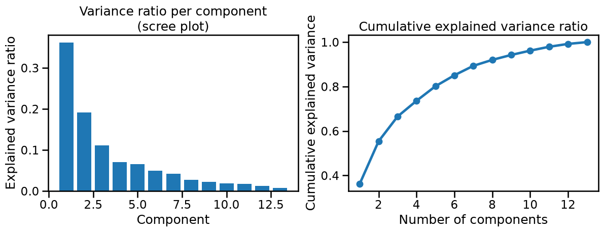
The bar chart on the left is called a scree plot. It shows how much new variance each additional component brings. The cumulative curve on the right shows the total variance captured as you include more components.
Historically, practitioners looked for an “elbow” in the scree plot, that is, the point where the bars stop dropping steeply and start to level off, similar to the elbow method in clustering. We will not dwell on it here because it is harder to interpret and less stable than the criteria we present below, but it is worth knowing the term.
Variance thresholds: 90% and 95%#
A common rule of thumb is to keep enough components to explain 90% or 95%
of the total variance. np.searchsorted finds the first index where the
cumulative variance crosses the threshold.
threshold_90 = np.searchsorted(cumulative, 0.90) + 1
threshold_95 = np.searchsorted(cumulative, 0.95) + 1

print(f"Components to reach 90% variance: {threshold_90}")
print(f"Components to reach 95% variance: {threshold_95}")
Components to reach 90% variance: 8
Components to reach 95% variance: 10
You can also let scikit-learn handle this directly by passing a float between
0 and 1 to the n_components parameter of PCA.
pipe_90 = make_pipeline(StandardScaler(), PCA(n_components=0.90))
pipe_90.fit(X)
print(
    f"n_components_ for 90% threshold: {pipe_90.named_steps['pca'].n_components_}"
)
n_components_ for 90% threshold: 8
Both thresholds are computed on the full dataset. But a PCA fitted on a
slightly different sample would produce slightly different components and
slightly different explained variance values. This raises a practical
question: if you deploy a model using threshold_90 components and claim
it retains 90% of the variance, how much variance does it actually retain
on a different sample of the same data?
We simulate this by fitting PCA on 20 random 50% subsamples and overlaying the resulting cumulative variance curves.
from sklearn.model_selection import train_test_split

n_splits = 20
split_explained = []

for random_state in range(n_splits):
    X_split, _ = train_test_split(X, train_size=0.5, random_state=random_state)
    pipe_split = make_pipeline(StandardScaler(), PCA())
    pipe_split.fit(X_split)
    split_explained.append(
        pipe_split.named_steps["pca"].explained_variance_ratio_
    )
fig, ax = plt.subplots(figsize=(8, 4))

for ev in split_explained:
    ax.plot(
        np.arange(1, len(ev) + 1), np.cumsum(ev), color="tab:blue", alpha=0.2
    )

ax.plot(
    components, cumulative, color="tab:blue", linewidth=2, label="Full dataset"
)
ax.axhline(0.90, color="tab:orange", linestyle="--", label="90%")
ax.axhline(0.95, color="tab:red", linestyle="--", label="95%")
ax.set_xlabel("Number of components")
ax.set_ylabel("Cumulative explained variance")
ax.set_title("Cumulative variance is not identical across subsamples")
ax.legend()

plt.show()
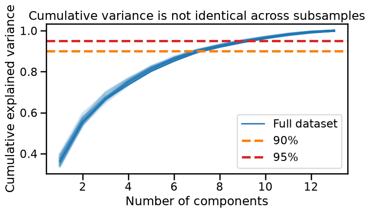
Each faint line is one subsample. The spread is most visible near the threshold lines, which means a fixed number of components does not guarantee exactly 90% or 95% variance retained. We can quantify this directly.
split_cumulative = np.array([np.cumsum(ev) for ev in split_explained])

for n_comp in [threshold_90, threshold_95]:
    values = split_cumulative[:, n_comp - 1] * 100
    print(
        f"{n_comp} components → {values.mean():.1f} ± {values.std():.1f}% "
        f"variance retained across splits"
    )
8 components → 92.6 ± 0.3% variance retained across splits
10 components → 96.6 ± 0.2% variance retained across splits
This is what you should report when justifying a component choice in a deployed model. Rather than stating “we retain 90% of the variance”, you can say “with N components, we retain X ± Y% of the variance across subsamples”, which is a more honest and informative claim.
The Kaiser criterion#
In the original Kaiser criterion (designed for factor analysis), you discard
components whose eigenvalue is below 1, meaning they explain less variance
than a single original variable would. The analog in PCA replaces the
raw eigenvalue threshold with its equivalent in variance ratio terms: keep
components that each explain more than 1/n_features of the total variance.
n_features = X.shape[1]
kaiser_threshold = 1 / n_features

print(f"Number of features: {n_features}")
print(f"Kaiser threshold (1/n_features): {kaiser_threshold:.4f}")
print(f"Components above threshold: {np.sum(explained > kaiser_threshold)}")

fig, ax = plt.subplots(figsize=(7, 4))
ax.bar(components, explained, label="Explained variance ratio")
ax.axhline(
    kaiser_threshold,
    color="tab:red",
    linestyle="--",
    label=f"Kaiser threshold (1/{n_features} ≈ {kaiser_threshold:.2f})",
)
ax.set_xlabel("Component")
ax.set_ylabel("Explained variance ratio")
ax.set_title(f"Kaiser criterion: keep components above 1/{n_features}")
ax.legend()
plt.show()
Number of features: 13
Kaiser threshold (1/n_features): 0.0769
Components above threshold: 3
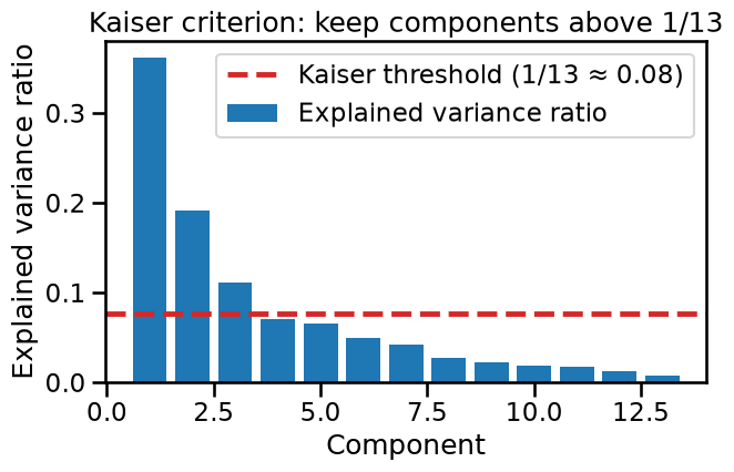
The Kaiser criterion does not require choosing a target variance level, which makes it easier to apply. One natural question is whether it also leads to more stable recommendations than the threshold approach. We overlay the same subsamples on the scree plot to find out.
fig, ax = plt.subplots(figsize=(7, 4))

for ev in split_explained:
    ax.plot(np.arange(1, len(ev) + 1), ev, color="tab:blue", alpha=0.2)

ax.plot(
    components, explained, color="tab:blue", linewidth=2, label="Full dataset"
)
ax.axhline(
    kaiser_threshold,
    color="tab:red",
    linestyle="--",
    label=f"Kaiser threshold (1/{n_features})",
)
ax.set_xlabel("Component")
ax.set_ylabel("Explained variance ratio")
ax.set_title("Kaiser criterion stability across subsamples")
ax.legend()
plt.show()
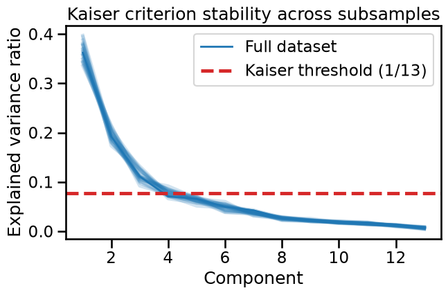
Notice that this curve reinforces the argument that finding an elbow depends heavily on the resampling and is not stable to resamplings.
Observe also that the curve has sampling variability near the 1/n_features
boundary. Because of that, this criterion does not lead to a unique choice for
the number of components for this dataset.
import pandas as pd

kaiser_n = np.sum(explained > kaiser_threshold)
kaiser_counts = [np.sum(ev > kaiser_threshold) for ev in split_explained]
ax = pd.Series(kaiser_counts).value_counts().sort_index().plot.bar(rot=0)
ax.set(
    title="Selected number of components across splits",
    xlabel="Number of components",
    ylabel="Counts",
)
plt.show()
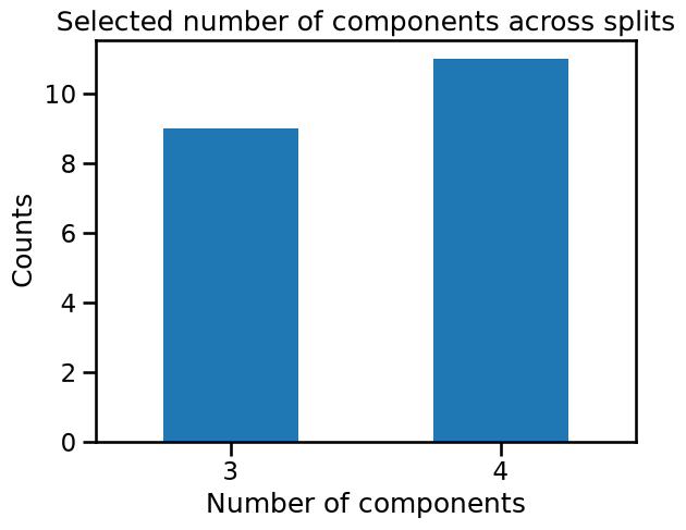
The Kaiser criterion suggests 3 or 4 components at almost the same rate.
Either choice is possible, but for the sake of this notebook, we retain
the latest value of kaiser_n and find how much of the total explained
variance it retains.
values = split_cumulative[:, kaiser_n - 1] * 100
print(
    f"{kaiser_n} components → {values.mean():.1f} ± {values.std():.1f}% "
    f"variance retained across splits"
)
3 components → 67.3 ± 1.2% variance retained across splits
Downstream check: does the component choice affect clustering?#
We now use KMeans as a downstream task to see whether the choice of
n_components has any practical impact. We fit the same range of cluster
counts under two pipelines: one using the Kaiser recommendation
(n_components=3) and one using the 90% threshold (n_components=8).
As in the clustering notebook, we plot the silhouette score against number of clusters and look for an elbow. Notice that silhouette is not comparable across different numbers of components, since the score depends on the space in which distances are computed, even if the score is normalized. We are not comparing the two curves against each other, instead we are checking whether each curve, read on its own, points to the same number of clusters.
We use the silhouette score and plot one curve per subsample, similarly to what we did in the clustering chapter of the Associate course. The two axes share the same y-axis range since the silhouette score has the same scale in both panels, which makes the comparison honest.
from sklearn.cluster import KMeans
from sklearn.metrics import silhouette_score

n_clusters_range = range(2, 11)

fig, axes = plt.subplots(1, 2, figsize=(12, 4), sharey=True)

for ax, n_components, label in zip(
    axes,
    [kaiser_n, threshold_90],
    [
        f"Kaiser ({kaiser_n} components)",
        f"90% threshold ({threshold_90} components)",
    ],
):
    pipe_km = make_pipeline(
        StandardScaler(),
        PCA(n_components=n_components),
        KMeans(random_state=0),
    )
    for random_state in range(1, 11):
        X_sub, _ = train_test_split(
            X, train_size=0.5, random_state=random_state
        )
        scores = []
        for k in n_clusters_range:
            pipe_km[-1].set_params(n_clusters=k)
            labels = pipe_km.fit_predict(X_sub)
            X_transformed = pipe_km[:-1].transform(X_sub)
            scores.append(silhouette_score(X_transformed, labels))
        ax.plot(n_clusters_range, scores, color="tab:blue", alpha=0.2)

    ax.set_xlabel("Number of clusters (n_clusters)")
    ax.set_ylabel("Silhouette score")
    ax.set_title(label)

plt.show()
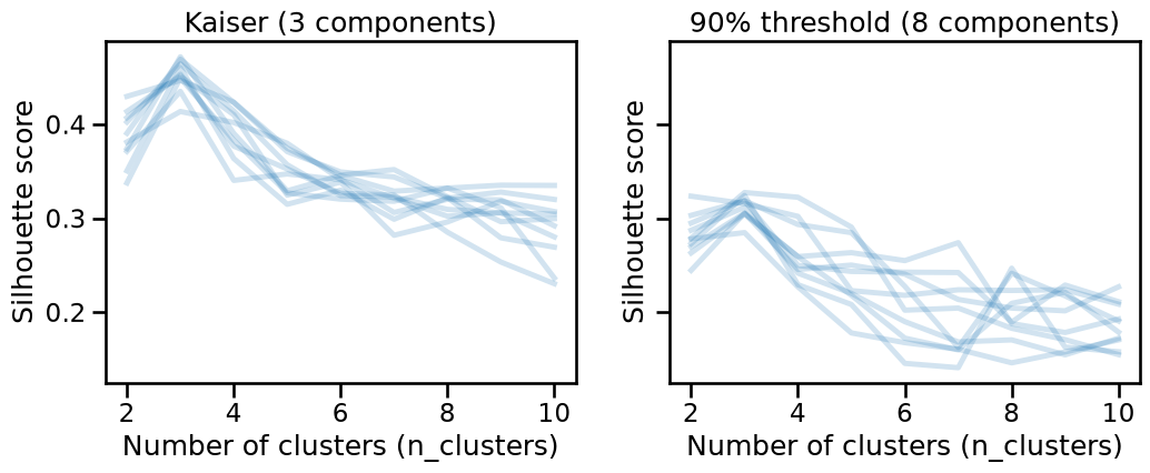
The two panels tell a different story. With the Kaiser components, the peak at 3 clusters is clear and consistent across all subsamples. With 8 components the curves are much more spread out and there is no clear consensus.
Keeping 92% variance is still capturing noise and therefore leading to high variance. Even in an unsupervised setting, we can conclude that the PCA step with 8 components is overfitting!
Notice also that the silhouette scores are also systematically lower in the
right panel. This is not because the quality of the clusters is worse in an
absolute sense, but because of the curse of dimensionality. In
high-dimensional spaces, all pairwise distances tend to concentrate around the
same value (a phenomenon known as distance concentration). As a result, the
within-cluster distance a and the nearest-cluster distance b become
increasingly similar, so the numerator b - a shrinks relative to max(a, b)
and the silhouette score is driven toward zero. For this reason we should not
compare the absolute level of the scores between the two panels. What matters
is the shape of each curve and where it peaks, not the y-axis value itself.
Key Takeaways#
The Kaiser criterion trades one arbitrary choice (the 90 - 95% level) for
another arbitrary choice (the 1/n_features rule). A priori neither is more
stable under resampling, but both allow us to make informed choices even in a
fully unsupervised pipeline.
In the case of supervised pipelines, prefer cross-validation to tune the number of components as you would do for any other hyperparameter.