Sample grouping

In this notebook we present the concept of sample groups. We use the handwritten digits dataset to highlight some surprising results.

from sklearn.datasets import load_digits

digits = load_digits()
data, target = digits.data, digits.target

We create a model consisting of a logistic regression classifier with a preprocessor to scale the data.

Note

Here we use a MinMaxScaler as we know that each pixel’s gray-scale is strictly bounded between 0 (white) and 16 (black). This makes MinMaxScaler more suited in this case than StandardScaler, as some pixels consistently have low variance (pixels at the borders might almost always be zero if most digits are centered in the image). Then, using StandardScaler can result in a very high scaled value due to division by a small number.

from sklearn.preprocessing import MinMaxScaler
from sklearn.linear_model import LogisticRegression
from sklearn.pipeline import make_pipeline

model = make_pipeline(MinMaxScaler(), LogisticRegression(max_iter=1_000))

The idea is to compare the estimated generalization performance using different cross-validation techniques and see how such estimations are impacted by underlying data structures. We first use a KFold cross-validation without shuffling the data.

from sklearn.model_selection import cross_val_score, KFold

cv = KFold(shuffle=False)
test_score_no_shuffling = cross_val_score(model, data, target, cv=cv, n_jobs=2)
print(
    "The average accuracy is "
    f"{test_score_no_shuffling.mean():.3f} ± "
    f"{test_score_no_shuffling.std():.3f}"
)

The average accuracy is 0.931 ± 0.027

Now, let’s repeat the experiment by shuffling the data within the cross-validation.

cv = KFold(shuffle=True)
test_score_with_shuffling = cross_val_score(
    model, data, target, cv=cv, n_jobs=2
)
print(
    "The average accuracy is "
    f"{test_score_with_shuffling.mean():.3f} ± "
    f"{test_score_with_shuffling.std():.3f}"
)

The average accuracy is 0.961 ± 0.005

We observe that shuffling the data improves the mean accuracy. We can go a little further and plot the distribution of the testing score. For such purpose we concatenate the test scores.

import pandas as pd

all_scores = pd.DataFrame(
    [test_score_no_shuffling, test_score_with_shuffling],
    index=["KFold without shuffling", "KFold with shuffling"],
).T

Let’s now plot the score distributions.

import matplotlib.pyplot as plt

all_scores.plot.hist(bins=16, edgecolor="black", alpha=0.7)
plt.xlim([0.8, 1.0])
plt.xlabel("Accuracy score")
plt.legend(bbox_to_anchor=(1.05, 0.8), loc="upper left")
_ = plt.title("Distribution of the test scores")

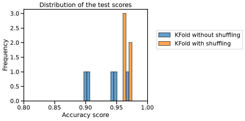
Shuffling the data results in a higher cross-validated test accuracy with less variance compared to when the data is not shuffled. It means that some specific fold leads to a low score in this case.

print(test_score_no_shuffling)

[0.94166667 0.89722222 0.94707521 0.96657382 0.90250696]

Thus, shuffling the data breaks the underlying structure and thus makes the classification task easier to our model. To get a better understanding, we can read the dataset description in more detail:

print(digits.DESCR)

.. _digits_dataset:

Optical recognition of handwritten digits dataset
--------------------------------------------------

**Data Set Characteristics:**

:Number of Instances: 1797
:Number of Attributes: 64
:Attribute Information: 8x8 image of integer pixels in the range 0..16.
:Missing Attribute Values: None
:Creator: E. Alpaydin (alpaydin '@' boun.edu.tr)
:Date: July; 1998

This is a copy of the test set of the UCI ML hand-written digits datasets
https://archive.ics.uci.edu/ml/datasets/Optical+Recognition+of+Handwritten+Digits

The data set contains images of hand-written digits: 10 classes where
each class refers to a digit.

Preprocessing programs made available by NIST were used to extract
normalized bitmaps of handwritten digits from a preprinted form. From a
total of 43 people, 30 contributed to the training set and different 13
to the test set. 32x32 bitmaps are divided into nonoverlapping blocks of
4x4 and the number of on pixels are counted in each block. This generates
an input matrix of 8x8 where each element is an integer in the range
0..16. This reduces dimensionality and gives invariance to small
distortions.

For info on NIST preprocessing routines, see M. D. Garris, J. L. Blue, G.
T. Candela, D. L. Dimmick, J. Geist, P. J. Grother, S. A. Janet, and C.
L. Wilson, NIST Form-Based Handprint Recognition System, NISTIR 5469,
1994.

|details-start|
**References**
|details-split|

- C. Kaynak (1995) Methods of Combining Multiple Classifiers and Their
  Applications to Handwritten Digit Recognition, MSc Thesis, Institute of
  Graduate Studies in Science and Engineering, Bogazici University.
- E. Alpaydin, C. Kaynak (1998) Cascading Classifiers, Kybernetika.
- Ken Tang and Ponnuthurai N. Suganthan and Xi Yao and A. Kai Qin.
  Linear dimensionalityreduction using relevance weighted LDA. School of
  Electrical and Electronic Engineering Nanyang Technological University.
  2005.
- Claudio Gentile. A New Approximate Maximal Margin Classification
  Algorithm. NIPS. 2000.

|details-end|

If we read carefully, 13 writers wrote the digits of our dataset, accounting for a total amount of 1797 samples. Thus, a writer wrote several times the same numbers. Let’s suppose that the writer samples are grouped. Subsequently, not shuffling the data will keep all writer samples together either in the training or the testing sets. Mixing the data will break this structure, and therefore digits written by the same writer will be available in both the training and testing sets.

Besides, a writer will usually tend to write digits in the same manner. Thus, our model will learn to identify a writer’s pattern for each digit instead of recognizing the digit itself.

We can solve this problem by ensuring that the data associated with a writer should either belong to the training or the testing set. Thus, we want to group samples for each writer.

Indeed, we can recover the groups by looking at the target variable.

target[:200]

array([0, 1, 2, 3, 4, 5, 6, 7, 8, 9, 0, 1, 2, 3, 4, 5, 6, 7, 8, 9, 0, 1,
       2, 3, 4, 5, 6, 7, 8, 9, 0, 9, 5, 5, 6, 5, 0, 9, 8, 9, 8, 4, 1, 7,
       7, 3, 5, 1, 0, 0, 2, 2, 7, 8, 2, 0, 1, 2, 6, 3, 3, 7, 3, 3, 4, 6,
       6, 6, 4, 9, 1, 5, 0, 9, 5, 2, 8, 2, 0, 0, 1, 7, 6, 3, 2, 1, 7, 4,
       6, 3, 1, 3, 9, 1, 7, 6, 8, 4, 3, 1, 4, 0, 5, 3, 6, 9, 6, 1, 7, 5,
       4, 4, 7, 2, 8, 2, 2, 5, 7, 9, 5, 4, 8, 8, 4, 9, 0, 8, 9, 8, 0, 1,
       2, 3, 4, 5, 6, 7, 8, 9, 0, 1, 2, 3, 4, 5, 6, 7, 8, 9, 0, 1, 2, 3,
       4, 5, 6, 7, 8, 9, 0, 9, 5, 5, 6, 5, 0, 9, 8, 9, 8, 4, 1, 7, 7, 3,
       5, 1, 0, 0, 2, 2, 7, 8, 2, 0, 1, 2, 6, 3, 3, 7, 3, 3, 4, 6, 6, 6,
       4, 9])

It might not be obvious at first, but there is a structure in the target: there is a repetitive pattern that always starts by some series of ordered digits from 0 to 9 followed by random digits at a certain point. If we look in detail, we see that there are 14 such patterns, always with around 130 samples each.

Even if it is not exactly corresponding to the 13 writers in the documentation (maybe one writer wrote two series of digits), we can make the hypothesis that each of these patterns corresponds to a different writer and thus a different group.

from itertools import count
import numpy as np

# defines the lower and upper bounds of sample indices
# for each writer
writer_boundaries = [
    0,
    130,
    256,
    386,
    516,
    646,
    776,
    915,
    1029,
    1157,
    1287,
    1415,
    1545,
    1667,
    1797,
]
groups = np.zeros_like(target)
lower_bounds = writer_boundaries[:-1]
upper_bounds = writer_boundaries[1:]

for group_id, lb, up in zip(count(), lower_bounds, upper_bounds):
    groups[lb:up] = group_id

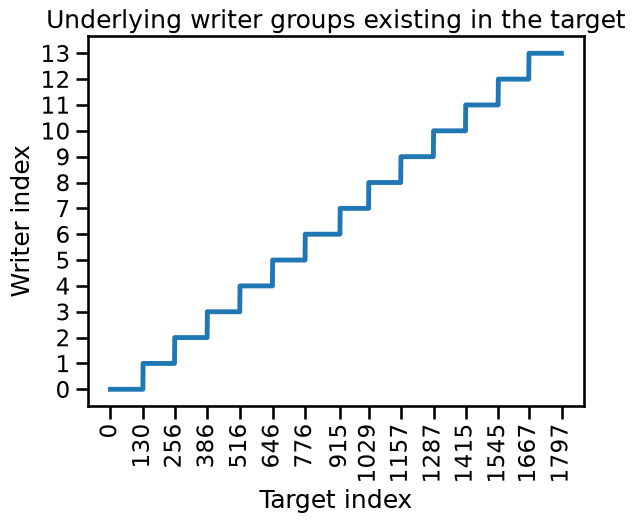
We can check the grouping by plotting the indices linked to writers’ ids.

plt.plot(groups)
plt.yticks(np.unique(groups))
plt.xticks(writer_boundaries, rotation=90)
plt.xlabel("Target index")
plt.ylabel("Writer index")
_ = plt.title("Underlying writer groups existing in the target")

Once we group the digits by writer, we can incorporate this information into the cross-validation process by using group-aware variations of the strategies we have explored in this course, for example, the GroupKFold strategy.

from sklearn.model_selection import GroupKFold

cv = GroupKFold()
test_score = cross_val_score(
    model, data, target, groups=groups, cv=cv, n_jobs=2
)
print(
    f"The average accuracy is {test_score.mean():.3f} ± {test_score.std():.3f}"
)

The average accuracy is 0.921 ± 0.021

We see that this strategy leads to a lower generalization performance than the other two techniques. However, this is the most reliable estimate if our goal is to evaluate the capabilities of the model to generalize to new unseen writers. In this sense, shuffling the dataset (or alternatively using the writers’ ids as a new feature) would lead the model to memorize the different writer’s particular handwriting.

all_scores = pd.DataFrame(
    [test_score_no_shuffling, test_score_with_shuffling, test_score],
    index=[
        "KFold without shuffling",
        "KFold with shuffling",
        "KFold with groups",
    ],
).T

all_scores.plot.hist(bins=16, edgecolor="black", alpha=0.7)
plt.xlim([0.8, 1.0])
plt.xlabel("Accuracy score")
plt.legend(bbox_to_anchor=(1.05, 0.8), loc="upper left")
_ = plt.title("Distribution of the test scores")

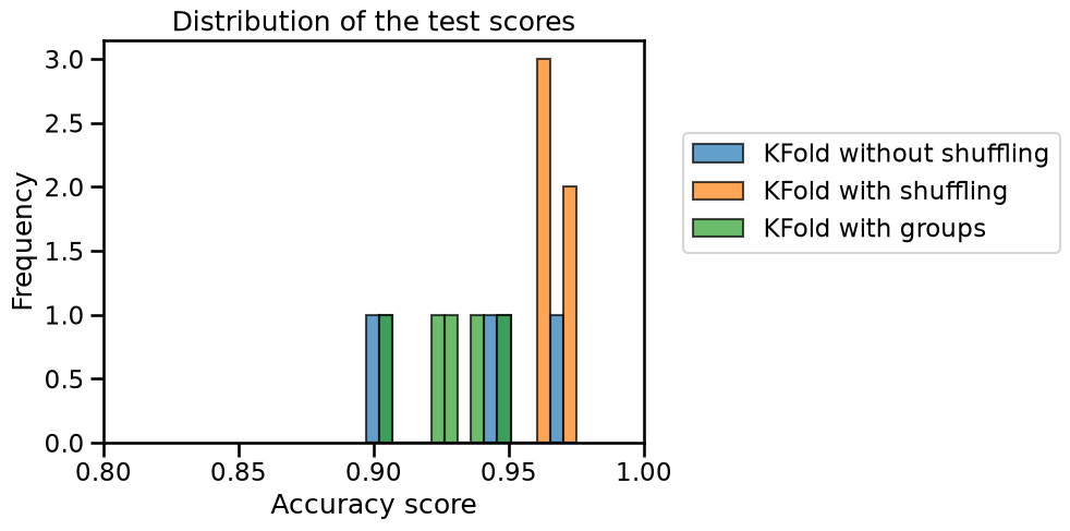
In conclusion, accounting for any sample grouping patterns is crucial when assessing a model’s ability to generalize to new groups. Without this consideration, the results may appear overly optimistic compared to the actual performance.

The interested reader can learn about other group-aware cross-validation techniques in the scikit-learn user guide.