📃 Solution for Exercise M4.01#
The aim of this exercise is two-fold:
understand the parametrization of a linear model;
quantify the fitting accuracy of a set of such models.
We will reuse part of the code of the course to:
load data;
create the function representing a linear model.
Prerequisites#
Data loading#
Note
If you want a deeper overview regarding this dataset, you can refer to the Appendix - Datasets description section at the end of this MOOC.
import pandas as pd

penguins = pd.read_csv("../datasets/penguins_regression.csv")
feature_name = "Flipper Length (mm)"
target_name = "Body Mass (g)"
data, target = penguins[[feature_name]], penguins[[target_name]]
Model definition#
def linear_model_flipper_mass(
    flipper_length, weight_flipper_length, intercept_body_mass
):
    """Linear model of the form y = a * x + b"""
    body_mass = weight_flipper_length * flipper_length + intercept_body_mass
    return body_mass
Main exercise#
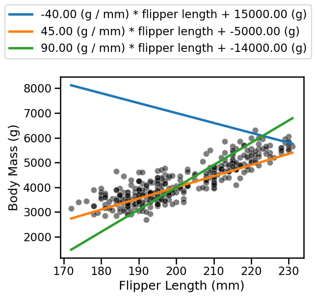
Define a vector weights = [...] and a vector intercepts = [...] of the
same length. Each pair of entries (weights[i], intercepts[i]) tags a
different model. Use these vectors along with the vector
flipper_length_range to plot several linear models that could possibly fit
our data. Use the above helper function to visualize both the models and the
real samples.
import numpy as np

flipper_length_range = np.linspace(data.min(), data.max(), num=300)
# solution
import matplotlib.pyplot as plt
import seaborn as sns

weights = [-40, 45, 90]
intercepts = [15000, -5000, -14000]

ax = sns.scatterplot(
    data=penguins, x=feature_name, y=target_name, color="black", alpha=0.5
)

label = "{0:.2f} (g / mm) * flipper length + {1:.2f} (g)"
for weight, intercept in zip(weights, intercepts):
    predicted_body_mass = linear_model_flipper_mass(
        flipper_length_range, weight, intercept
    )

    ax.plot(
        flipper_length_range,
        predicted_body_mass,
        label=label.format(weight, intercept),
    )
_ = ax.legend(loc="center left", bbox_to_anchor=(-0.25, 1.25), ncol=1)

In the previous question, you were asked to create several linear models. The visualization allowed you to qualitatively assess if a model was better than another.
Now, you should come up with a quantitative measure which indicates the
goodness of fit of each linear model and allows you to select the best model.
Define a function goodness_fit_measure(true_values, predictions) that takes
as inputs the true target values and the predictions and returns a single
scalar as output.
# solution
def goodness_fit_measure(true_values, predictions):
    # we compute the error between the true values and the predictions of our
    # model
    errors = true_values - predictions
    # We have several possible strategies to reduce all errors to a single value.
    # Computing the mean error (sum divided by the number of element) might seem
    # like a good solution. However, we have negative errors that will misleadingly
    # reduce the mean error. Therefore, we can either square each
    # error or take the absolute value: these metrics are known as mean
    # squared error (MSE) and mean absolute error (MAE). Let's use the MAE here
    # as an example.
    return np.mean(np.abs(errors))
You can now copy and paste the code below to show the goodness of fit for each model.
for model_idx, (weight, intercept) in enumerate(zip(weights, intercepts)):
    target_predicted = linear_model_flipper_mass(data, weight, intercept)
    print(f"Model #{model_idx}:")
    print(f"{weight:.2f} (g / mm) * flipper length + {intercept:.2f} (g)")
    print(f"Error: {goodness_fit_measure(target, target_predicted):.3f}\n")
# solution
for model_idx, (weight, intercept) in enumerate(zip(weights, intercepts)):
    target_predicted = linear_model_flipper_mass(data, weight, intercept)
    print(f"Model #{model_idx}:")
    print(f"{weight:.2f} (g / mm) * flipper length + {intercept:.2f} (g)")
    print(f"Error: {goodness_fit_measure(target, target_predicted):.3f}\n")
Model #0:
-40.00 (g / mm) * flipper length + 15000.00 (g)
Error: nan

Model #1:
45.00 (g / mm) * flipper length + -5000.00 (g)
Error: nan

Model #2:
90.00 (g / mm) * flipper length + -14000.00 (g)
Error: nan

