Stratification

In the previous notebooks, we always used either a default KFold or a ShuffleSplit cross-validation strategies to iteratively split our dataset. However, you should not assume that these approaches are always the best option: some other cross-validation strategies might be better adapted to your problem.

Let’s start with the concept of stratification by giving an example where we can get into trouble if we are not careful. Let’s load the iris dataset.

from sklearn.datasets import load_iris

data, target = load_iris(as_frame=True, return_X_y=True)

At this point, we create a basic machine-learning model: a logistic regression. We expect this model to work quite well on the iris dataset since this is a toy dataset.

from sklearn.preprocessing import StandardScaler
from sklearn.linear_model import LogisticRegression
from sklearn.pipeline import make_pipeline

model = make_pipeline(StandardScaler(), LogisticRegression())

Once the model is created, we can evaluate it using cross-validation. We start by using the KFold strategy.

Let’s review how this strategy works. For such purpose, we define a dataset with nine samples and split the dataset into three folds (i.e. n_splits=3).

import numpy as np
from sklearn.model_selection import KFold

data_random = np.random.randn(9, 1)
cv = KFold(n_splits=3)
for train_index, test_index in cv.split(data_random):
    print("TRAIN:", train_index, "TEST:", test_index)

TRAIN: [3 4 5 6 7 8] TEST: [0 1 2]
TRAIN: [0 1 2 6 7 8] TEST: [3 4 5]
TRAIN: [0 1 2 3 4 5] TEST: [6 7 8]

By defining three splits, we use three samples (1-fold) for testing and six (2-folds) for training each time. KFold does not shuffle by default. It means that the three first samples are selected for the testing set at the first split, then the three next three samples for the second split, and the three next for the last split. In the end, all samples have been used in testing at least once among the different splits.

Now, let’s apply this strategy to check the generalization performance of our model.

from sklearn.model_selection import cross_validate

cv = KFold(n_splits=3)
results = cross_validate(model, data, target, cv=cv)
test_score = results["test_score"]
print(
    f"The average accuracy is {test_score.mean():.3f} ± {test_score.std():.3f}"
)

The average accuracy is 0.000 ± 0.000

It is a real surprise that our model cannot correctly classify any sample in any cross-validation split. We now check our target’s value to understand the issue.

import matplotlib.pyplot as plt

target.plot()
plt.xlabel("Sample index")
plt.ylabel("Class")
plt.yticks(target.unique())
_ = plt.title("Class value in target y")

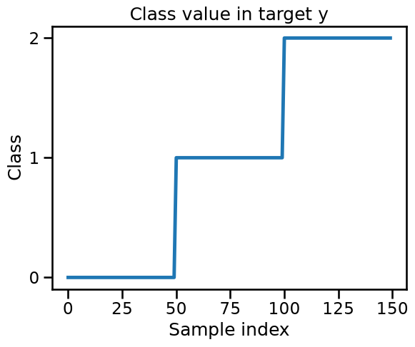
We see that the target vector target is ordered. This has some unexpected consequences when using the KFold cross-validation. To illustrate the consequences, we show the class count in each fold of the cross-validation in the train and test set.

Let’s compute the class counts for both the training and testing sets using the KFold cross-validation, and plot these information in a bar plot.

We iterate given the number of split and check how many samples of each are present in the training and testing set. We then store the information into two distinct lists; one for the training set and one for the testing set.

import pandas as pd

n_splits = 3
cv = KFold(n_splits=n_splits)

train_cv_counts = []
test_cv_counts = []
for fold_idx, (train_idx, test_idx) in enumerate(cv.split(data, target)):
    target_train, target_test = target.iloc[train_idx], target.iloc[test_idx]

    train_cv_counts.append(target_train.value_counts())
    test_cv_counts.append(target_test.value_counts())

To plot the information on a single figure, we concatenate the information regarding the fold within the same dataset.

train_cv_counts = pd.concat(
    train_cv_counts, axis=1, keys=[f"Fold #{idx}" for idx in range(n_splits)]
)
train_cv_counts.index.name = "Class label"
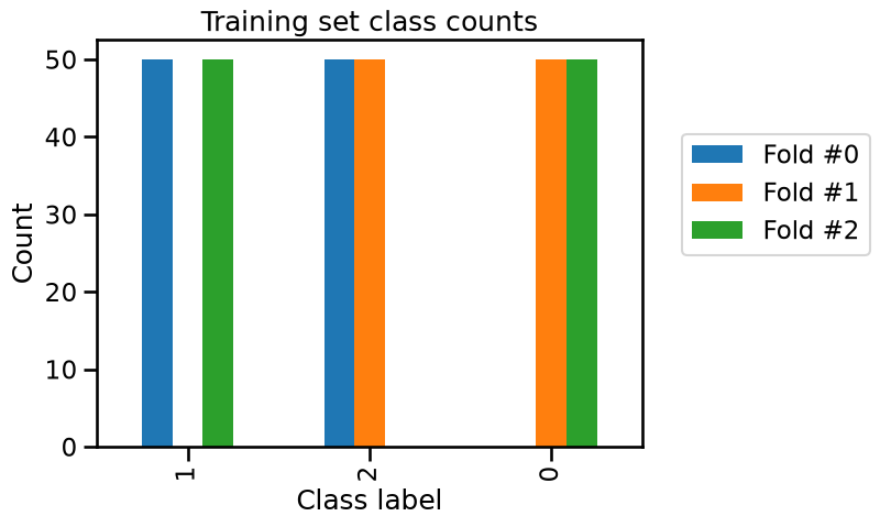
train_cv_counts

	Fold #0	Fold #1	Fold #2
Class label
1	50.0	NaN	50.0
2	50.0	50.0	NaN
0	NaN	50.0	50.0

test_cv_counts = pd.concat(
    test_cv_counts, axis=1, keys=[f"Fold #{idx}" for idx in range(n_splits)]
)
test_cv_counts.index.name = "Class label"
test_cv_counts

	Fold #0	Fold #1	Fold #2
Class label
0	50.0	NaN	NaN
1	NaN	50.0	NaN
2	NaN	NaN	50.0

Now we can represent graphically this information with bar plots.

train_cv_counts.plot.bar()
plt.legend(bbox_to_anchor=(1.05, 0.8), loc="upper left")
plt.ylabel("Count")
_ = plt.title("Training set class counts")

test_cv_counts.plot.bar()
plt.legend(bbox_to_anchor=(1.05, 0.8), loc="upper left")
plt.ylabel("Count")
_ = plt.title("Test set class counts")

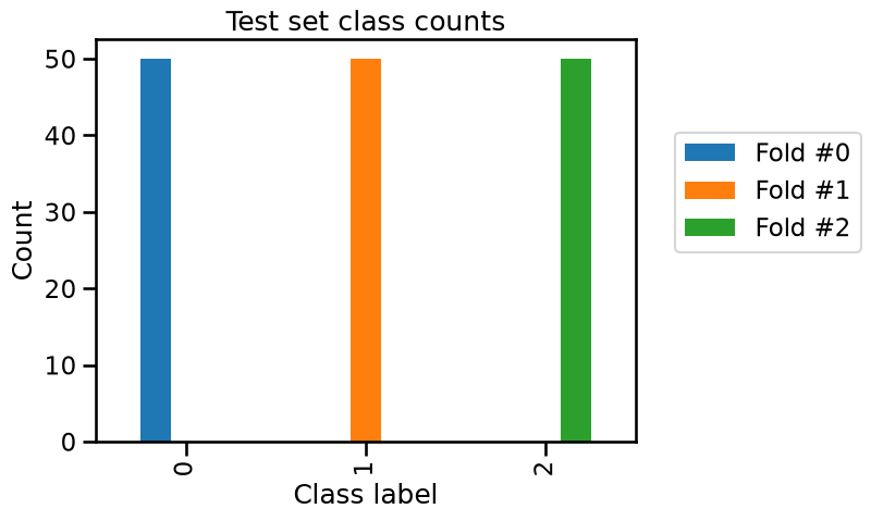
We can confirm that in each fold, only two of the three classes are present in the training set and all samples of the remaining class is used as a test set. So our model is unable to predict this class that was unseen during the training stage.

One possibility to solve the issue is to shuffle the data before splitting the data into three groups.

cv = KFold(n_splits=3, shuffle=True, random_state=0)
results = cross_validate(model, data, target, cv=cv)
test_score = results["test_score"]
print(
    f"The average accuracy is {test_score.mean():.3f} ± {test_score.std():.3f}"
)

The average accuracy is 0.953 ± 0.009

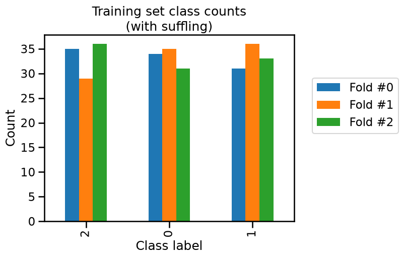
We get results that are closer to what we would expect with an accuracy above 90%. Now that we solved our first issue, it would be interesting to check if the class frequency in the training and testing set is equal to our original set’s class frequency. It would ensure that we are training and testing our model with a class distribution that we would encounter in production.

train_cv_counts = []
test_cv_counts = []
for fold_idx, (train_idx, test_idx) in enumerate(cv.split(data, target)):
    target_train, target_test = target.iloc[train_idx], target.iloc[test_idx]

    train_cv_counts.append(target_train.value_counts())
    test_cv_counts.append(target_test.value_counts())
train_cv_counts = pd.concat(
    train_cv_counts, axis=1, keys=[f"Fold #{idx}" for idx in range(n_splits)]
)
test_cv_counts = pd.concat(
    test_cv_counts, axis=1, keys=[f"Fold #{idx}" for idx in range(n_splits)]
)
train_cv_counts.index.name = "Class label"
test_cv_counts.index.name = "Class label"

train_cv_counts.plot.bar()
plt.legend(bbox_to_anchor=(1.05, 0.8), loc="upper left")
plt.ylabel("Count")
_ = plt.title("Training set class counts\n(with suffling)")

test_cv_counts.plot.bar()
plt.legend(bbox_to_anchor=(1.05, 0.8), loc="upper left")
plt.ylabel("Count")
_ = plt.title("Test set class counts\n(with suffling)")

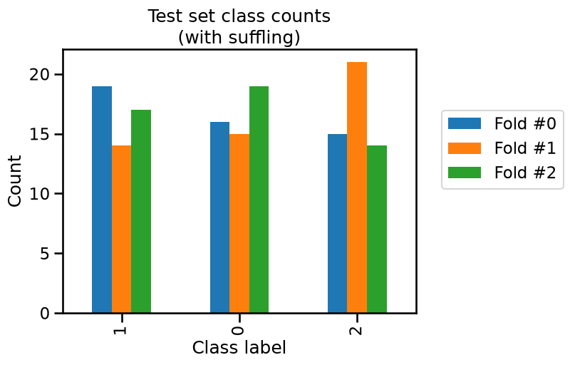
We see that neither the training and testing sets have the same class frequencies as our original dataset because the count for each class is varying a little.

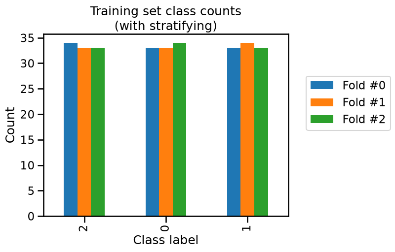
However, one might want to split our data by preserving the original class frequencies: we want to stratify our data by class. In scikit-learn, some cross-validation strategies implement the stratification; they contain Stratified in their names.

from sklearn.model_selection import StratifiedKFold

cv = StratifiedKFold(n_splits=3)

results = cross_validate(model, data, target, cv=cv)
test_score = results["test_score"]
print(
    f"The average accuracy is {test_score.mean():.3f} ± {test_score.std():.3f}"
)

The average accuracy is 0.967 ± 0.009

train_cv_counts = []
test_cv_counts = []
for fold_idx, (train_idx, test_idx) in enumerate(cv.split(data, target)):
    target_train, target_test = target.iloc[train_idx], target.iloc[test_idx]

    train_cv_counts.append(target_train.value_counts())
    test_cv_counts.append(target_test.value_counts())
train_cv_counts = pd.concat(
    train_cv_counts, axis=1, keys=[f"Fold #{idx}" for idx in range(n_splits)]
)
test_cv_counts = pd.concat(
    test_cv_counts, axis=1, keys=[f"Fold #{idx}" for idx in range(n_splits)]
)
train_cv_counts.index.name = "Class label"
test_cv_counts.index.name = "Class label"

train_cv_counts.plot.bar()
plt.legend(bbox_to_anchor=(1.05, 0.8), loc="upper left")
plt.ylabel("Count")
_ = plt.title("Training set class counts\n(with stratifying)")

test_cv_counts.plot.bar()
plt.legend(bbox_to_anchor=(1.05, 0.8), loc="upper left")
plt.ylabel("Count")
_ = plt.title("Test set class counts\n(with stratifying)")

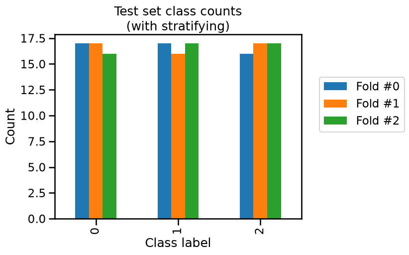
In this case, we observe that the class counts are very close both in the train set and the test set. The difference is due to the small number of samples in the iris dataset.

In other words, stratifying is more effective than just shuffling when it comes to making sure that the distributions of classes in all the folds are representative of the entire dataset. As training and testing folds have similar class distributions, stratifying leads to a more realistic measure of the model’s ability to generalize. This is specially important when the performance metrics depend on the proportion of the positive class, as we will see in a future notebook.

The interested reader can learn about other stratified cross-validation techniques in the scikit-learn user guide.