Regression

In this notebook, we present the metrics that can be used in regression.

A set of metrics are dedicated to regression. Indeed, classification metrics cannot be used to evaluate the generalization performance of regression models because there is a fundamental difference between their target type target: it is a continuous variable in regression, while a discrete variable in classification.

We use the Ames housing dataset. The goal is to predict the price of houses in the city of Ames, Iowa. As with classification, we only use a single train-test split to focus solely on the regression metrics.

import pandas as pd
import numpy as np

ames_housing = pd.read_csv("../datasets/house_prices.csv")
data = ames_housing.drop(columns="SalePrice")
target = ames_housing["SalePrice"]
data = data.select_dtypes(np.number)
target /= 1000

Note

If you want a deeper overview regarding this dataset, you can refer to the Appendix - Datasets description section at the end of this MOOC.

Let’s start by splitting our dataset intro a train and test set.

from sklearn.model_selection import train_test_split

data_train, data_test, target_train, target_test = train_test_split(
    data, target, shuffle=True, random_state=0
)

Some machine learning models are designed to be solved as an optimization problem: minimizing an error (also known as the loss function) using a training set. A basic loss function used in regression is the mean squared error (MSE). Thus, this metric is sometimes used to evaluate the model since it is optimized by said model.

We give an example using a linear regression model.

from sklearn.linear_model import LinearRegression
from sklearn.metrics import mean_squared_error

regressor = LinearRegression()
regressor.fit(data_train, target_train)
target_predicted = regressor.predict(data_train)

print(
    "Mean squared error on the training set: "
    f"{mean_squared_error(target_train, target_predicted):.3f}"
)

Mean squared error on the training set: 996.902

Our linear regression model is minimizing the mean squared error on the training set. It means that there is no other set of coefficients which decreases the error.

Then, we can compute the mean squared error on the test set.

target_predicted = regressor.predict(data_test)

print(
    "Mean squared error on the testing set: "
    f"{mean_squared_error(target_test, target_predicted):.3f}"
)

Mean squared error on the testing set: 2064.736

The raw MSE can be difficult to interpret. One way is to rescale the MSE by the variance of the target. This score is known as the \(R^2\) also called the coefficient of determination. Indeed, this is the default score used in scikit-learn by calling the method score.

regressor.score(data_test, target_test)

0.6872520581075443

The \(R^2\) score represents the proportion of variance of the target that is explained by the independent variables in the model. The best score possible is 1 but there is no lower bound. However, a model that predicts the expected value of the target would get a score of 0.

from sklearn.dummy import DummyRegressor

dummy_regressor = DummyRegressor(strategy="mean")
dummy_regressor.fit(data_train, target_train)
print(
    "R2 score for a regressor predicting the mean:"
    f"{dummy_regressor.score(data_test, target_test):.3f}"
)

R2 score for a regressor predicting the mean:-0.000

The \(R^2\) score gives insight into the quality of the model’s fit. However, this score cannot be compared from one dataset to another and the value obtained does not have a meaningful interpretation relative the original unit of the target. If we wanted to get an interpretable score, we would be interested in the median or mean absolute error.

from sklearn.metrics import mean_absolute_error

target_predicted = regressor.predict(data_test)
print(
    "Mean absolute error: "
    f"{mean_absolute_error(target_test, target_predicted):.3f} k$"
)

Mean absolute error: 22.608 k$

By computing the mean absolute error, we can interpret that our model is predicting on average 22.6 k$ away from the true house price. A disadvantage of this metric is that the mean can be impacted by large error. For some applications, we might not want these large errors to have such a big influence on our metric. In this case we can use the median absolute error.

from sklearn.metrics import median_absolute_error

print(
    "Median absolute error: "
    f"{median_absolute_error(target_test, target_predicted):.3f} k$"
)

Median absolute error: 14.137 k$

The mean absolute error (or median absolute error) still have a known limitation: committing an error of 50 k$ for a house valued at 50 k$ has the same impact than committing an error of 50 k$ for a house valued at 500 k$. Indeed, the mean absolute error is not relative.

The mean absolute percentage error introduce this relative scaling.

from sklearn.metrics import mean_absolute_percentage_error

print(
    "Mean absolute percentage error: "
    f"{mean_absolute_percentage_error(target_test, target_predicted) * 100:.3f} %"
)

Mean absolute percentage error: 13.574 %

In addition to using metrics, we can visualize the results by plotting the predicted values versus the true values.

In an ideal scenario where all variations in the target could be perfectly explained by the obseved features (i.e. without any unobserved factors of variations), and we have chosen an optimal model, we would expect all predictions to fall along the diagonal line of the first plot below.

In the real life, this is almost never the case: some unknown fraction of the variations in the target cannot be explained by variations in data: they stem from external factors not represented by the observed features.

Therefore, the best we can hope for is that our model’s predictions form a cloud of points symmetrically distributed around the diagonal line, ideally close enough to it for the model to be useful.

To gain more insight, it can be helpful to plot the residuals, which represent the difference between the actual and predicted values, against the predicted values. This is shown in the second plot.

Residual plots make it easier to assess if the residuals exhibit a variance independent of the target values or if there is any systematic bias of the model associated with the lowest or highest predicted values.

import matplotlib.pyplot as plt
from sklearn.metrics import PredictionErrorDisplay

fig, axs = plt.subplots(ncols=2, figsize=(13, 5))

PredictionErrorDisplay.from_predictions(
    y_true=target_test,
    y_pred=target_predicted,
    kind="actual_vs_predicted",
    scatter_kwargs={"alpha": 0.5},
    ax=axs[0],
)
axs[0].axis("square")
axs[0].set_xlabel("Predicted values (k$)")
axs[0].set_ylabel("True values (k$)")

PredictionErrorDisplay.from_predictions(
    y_true=target_test,
    y_pred=target_predicted,
    kind="residual_vs_predicted",
    scatter_kwargs={"alpha": 0.5},
    ax=axs[1],
)
axs[1].axis("square")
axs[1].set_xlabel("Predicted values (k$)")
axs[1].set_ylabel("Residual values (k$)")

_ = fig.suptitle(
    "Regression using a model\nwithout target transformation", y=1.1
)

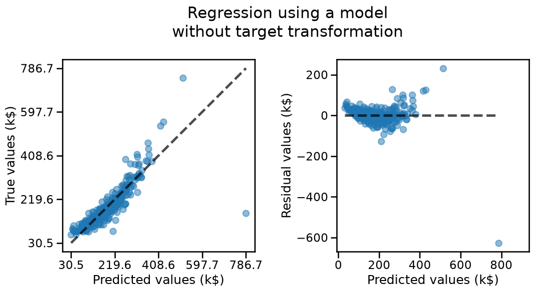
On these plots, we see that our model tends to under-estimate the price of the house both for the lowest and large True price values. This means that the residuals still hold some structure typically visible as the “banana” or “smile” shape of the residual plot. This is often a clue that our model could be improved, either by transforming the features, the target or sometimes changing the model type or its parameters. In this case let’s try to see if the model would benefit from a target transformation that monotonically reshapes the target variable to follow a normal distribution.

from sklearn.preprocessing import QuantileTransformer
from sklearn.compose import TransformedTargetRegressor

transformer = QuantileTransformer(
    n_quantiles=900, output_distribution="normal"
)
model_transformed_target = TransformedTargetRegressor(
    regressor=regressor, transformer=transformer
)
model_transformed_target.fit(data_train, target_train)
target_predicted = model_transformed_target.predict(data_test)

fig, axs = plt.subplots(ncols=2, figsize=(13, 5))

PredictionErrorDisplay.from_predictions(
    y_true=target_test,
    y_pred=target_predicted,
    kind="actual_vs_predicted",
    scatter_kwargs={"alpha": 0.5},
    ax=axs[0],
)
axs[0].axis("square")
axs[0].set_xlabel("Predicted values (k$)")
axs[0].set_ylabel("True values (k$)")

PredictionErrorDisplay.from_predictions(
    y_true=target_test,
    y_pred=target_predicted,
    kind="residual_vs_predicted",
    scatter_kwargs={"alpha": 0.5},
    ax=axs[1],
)
axs[1].axis("square")
axs[1].set_xlabel("Predicted values (k$)")
axs[1].set_ylabel("Residual values (k$)")

_ = fig.suptitle(
    "Regression using a model that\ntransforms the target before fitting",
    y=1.1,
)

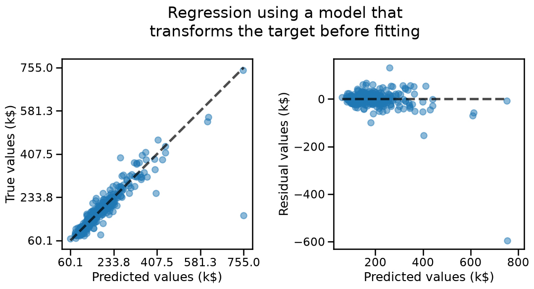
The model with the transformed target seems to exhibit fewer structure in its residuals: over-estimation and under-estimation errors seems to be more balanced.

We can confirm this by computing the previously mentioned metrics and observe that they all improved w.r.t. the linear regression model without the target transformation.

print(
    "Mean absolute error: "
    f"{mean_absolute_error(target_test, target_predicted):.3f} k$"
)
print(
    "Median absolute error: "
    f"{median_absolute_error(target_test, target_predicted):.3f} k$"
)
print(
    "Mean absolute percentage error: "
    f"{mean_absolute_percentage_error(target_test, target_predicted):.2%}"
)

Mean absolute error: 17.406 k$
Median absolute error: 10.327 k$
Mean absolute percentage error: 9.92%

While a common practice, performing such a target transformation for linear regression is often disapproved by statisticians. It is mathematically more justified to instead adapt the loss function of the regression model itself, for instance by fitting a PoissonRegressor or a TweedieRegressor model instead of LinearRegression. In particular those models indeed use an internal “log link” function that makes them more suited for this kind of positive-only target data distributions, but this analysis is beyond the scope of this MOOC.

The interested readers are encouraged to learn more about those models, in particular by reading their respective docstrings and the linked sections in the scikit-learn user guide reachable from the links above.