Effect of the sample size in cross-validation#
In the previous notebook, we presented the general cross-validation framework and how to assess if a predictive model is underfitting, overfitting, or generalizing. Besides these aspects, it is also important to understand how the different errors are influenced by the number of samples available.
In this notebook, we will show this aspect by looking at the variability of the different errors.
Let’s first load the data and create the same model as in the previous notebook.
from sklearn.datasets import fetch_california_housing

housing = fetch_california_housing(as_frame=True)
data, target = housing.data, housing.target
target *= 100  # rescale the target in k$
Note
If you want a deeper overview regarding this dataset, you can refer to the Appendix - Datasets description section at the end of this MOOC.
from sklearn.tree import DecisionTreeRegressor

regressor = DecisionTreeRegressor()
Learning curve#
To understand the impact of the number of samples available for training on the generalization performance of a predictive model, it is possible to synthetically reduce the number of samples used to train the predictive model and check the training and testing errors.
Therefore, we can vary the number of samples in the training set and repeat the experiment. The training and testing scores can be plotted similarly to the validation curve, but instead of varying a hyperparameter, we vary the number of training samples. This curve is called the learning curve.
It gives information regarding the benefit of adding new training samples to improve a model’s generalization performance.
Let’s compute the learning curve for a decision tree and vary the proportion of the training set from 10% to 100%.
import numpy as np

train_sizes = np.linspace(0.1, 1.0, num=5, endpoint=True)
train_sizes
array([0.1 , 0.325, 0.55 , 0.775, 1. ])
We will use a ShuffleSplit cross-validation to assess our predictive model.
from sklearn.model_selection import ShuffleSplit

cv = ShuffleSplit(n_splits=30, test_size=0.2)
Now, we are all set to carry out the experiment.
from sklearn.model_selection import LearningCurveDisplay

display = LearningCurveDisplay.from_estimator(
    regressor,
    data,
    target,
    train_sizes=train_sizes,
    cv=cv,
    score_type="both",  # both train and test errors
    scoring="neg_mean_absolute_error",
    negate_score=True,  # to use when metric starts with "neg_"
    score_name="Mean absolute error (k$)",
    std_display_style="errorbar",
    n_jobs=2,
)
_ = display.ax_.set(xscale="log", title="Learning curve for decision tree")
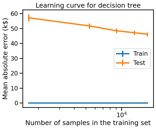
Looking at the training error alone, we see that we get an error of 0 k$. It means that the trained model (i.e. decision tree) is clearly overfitting the training data.
Looking at the testing error alone, we observe that the more samples are added into the training set, the lower the testing error becomes. Also, we are searching for the plateau of the testing error for which there is no benefit to adding samples anymore or assessing the potential gain of adding more samples into the training set.
If the testing error plateaus despite adding more training samples, it’s
possible that the model has achieved its optimal performance. In this case,
using a more expressive model might help reduce the error further. Otherwise,
the error may have reached the Bayes error rate, the theoretical minimum error
due to inherent uncertainty not resolved by the available data. This minimum error is
non-zero whenever some of the variation of the target variable y depends on
external factors not fully observed in the features available in X, which is
almost always the case in practice.
Summary#
In the notebook, we learnt:
the influence of the number of samples in a dataset, especially on the variability of the errors reported when running the cross-validation;
about the learning curve, which is a visual representation of the capacity of a model to improve by adding new samples.