The Ames housing dataset#
In this notebook, we will quickly present the “Ames housing” dataset. We will see that this dataset is similar to the “California housing” dataset. However, it is more complex to handle: it contains missing data and both numerical and categorical features.
This dataset is located in the datasets directory. It is stored in a comma
separated value (CSV) file. As previously mentioned, we are aware that the
dataset contains missing values. The character "?" is used as a missing
value marker.
We will open the dataset and specify the missing value marker such that they will be parsed by pandas when opening the file.
import pandas as pd

ames_housing = pd.read_csv("../datasets/house_prices.csv", na_values="?")
ames_housing = ames_housing.drop(columns="Id")
We can have a first look at the available columns in this dataset.
ames_housing.head()
| MSSubClass | MSZoning | LotFrontage | LotArea | Street | Alley | LotShape | LandContour | Utilities | LotConfig | ... | PoolArea | PoolQC | Fence | MiscFeature | MiscVal | MoSold | YrSold | SaleType | SaleCondition | SalePrice | |
|---|---|---|---|---|---|---|---|---|---|---|---|---|---|---|---|---|---|---|---|---|---|
| 0 | 60 | RL | 65.0 | 8450 | Pave | NaN | Reg | Lvl | AllPub | Inside | ... | 0 | NaN | NaN | NaN | 0 | 2 | 2008 | WD | Normal | 208500 |
| 1 | 20 | RL | 80.0 | 9600 | Pave | NaN | Reg | Lvl | AllPub | FR2 | ... | 0 | NaN | NaN | NaN | 0 | 5 | 2007 | WD | Normal | 181500 |
| 2 | 60 | RL | 68.0 | 11250 | Pave | NaN | IR1 | Lvl | AllPub | Inside | ... | 0 | NaN | NaN | NaN | 0 | 9 | 2008 | WD | Normal | 223500 |
| 3 | 70 | RL | 60.0 | 9550 | Pave | NaN | IR1 | Lvl | AllPub | Corner | ... | 0 | NaN | NaN | NaN | 0 | 2 | 2006 | WD | Abnorml | 140000 |
| 4 | 60 | RL | 84.0 | 14260 | Pave | NaN | IR1 | Lvl | AllPub | FR2 | ... | 0 | NaN | NaN | NaN | 0 | 12 | 2008 | WD | Normal | 250000 |
5 rows × 80 columns
We see that the last column named "SalePrice" is indeed the target that we
would like to predict. So we will split our dataset into two variables
containing the data and the target.
target_name = "SalePrice"
data, target = (
    ames_housing.drop(columns=target_name),
    ames_housing[target_name],
)
Let’s have a quick look at the target before to focus on the data.
target.head()
0    208500
1    181500
2    223500
3    140000
4    250000
Name: SalePrice, dtype: int64
We see that the target contains continuous value. It corresponds to the price of a house in $. We can have a look at the target distribution.
import matplotlib.pyplot as plt

target.plot.hist(bins=20, edgecolor="black")
plt.xlabel("House price in $")
_ = plt.title("Distribution of the house price \nin Ames")
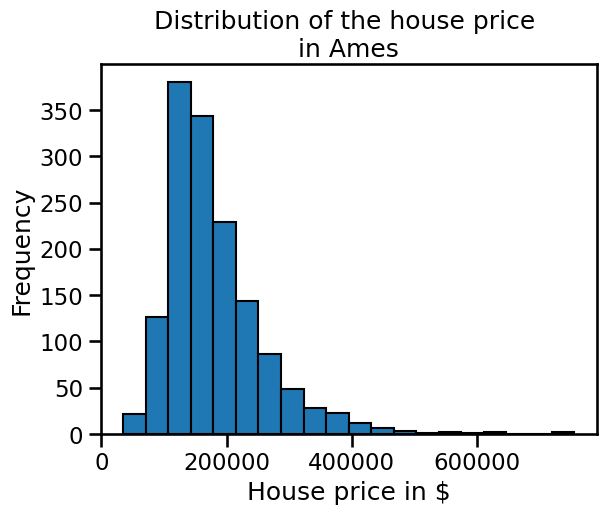
We see that the distribution has a long tail. It means that most of the house are normally distributed but a couple of houses have a higher than normal value. It could be critical to take this peculiarity into account when designing a predictive model.
Now, we can have a look at the available data that we could use to predict house prices.
data.info()
<class 'pandas.core.frame.DataFrame'>
RangeIndex: 1460 entries, 0 to 1459
Data columns (total 79 columns):
 #   Column         Non-Null Count  Dtype
---  ------         --------------  -----
 0   MSSubClass     1460 non-null   int64
 1   MSZoning       1460 non-null   object
 2   LotFrontage    1201 non-null   float64
 3   LotArea        1460 non-null   int64
 4   Street         1460 non-null   object
 5   Alley          91 non-null     object
 6   LotShape       1460 non-null   object
 7   LandContour    1460 non-null   object
 8   Utilities      1460 non-null   object
 9   LotConfig      1460 non-null   object
 10  LandSlope      1460 non-null   object
 11  Neighborhood   1460 non-null   object
 12  Condition1     1460 non-null   object
 13  Condition2     1460 non-null   object
 14  BldgType       1460 non-null   object
 15  HouseStyle     1460 non-null   object
 16  OverallQual    1460 non-null   int64
 17  OverallCond    1460 non-null   int64
 18  YearBuilt      1460 non-null   int64
 19  YearRemodAdd   1460 non-null   int64
 20  RoofStyle      1460 non-null   object
 21  RoofMatl       1460 non-null   object
 22  Exterior1st    1460 non-null   object
 23  Exterior2nd    1460 non-null   object
 24  MasVnrType     588 non-null    object
 25  MasVnrArea     1452 non-null   float64
 26  ExterQual      1460 non-null   object
 27  ExterCond      1460 non-null   object
 28  Foundation     1460 non-null   object
 29  BsmtQual       1423 non-null   object
 30  BsmtCond       1423 non-null   object
 31  BsmtExposure   1422 non-null   object
 32  BsmtFinType1   1423 non-null   object
 33  BsmtFinSF1     1460 non-null   int64
 34  BsmtFinType2   1422 non-null   object
 35  BsmtFinSF2     1460 non-null   int64
 36  BsmtUnfSF      1460 non-null   int64
 37  TotalBsmtSF    1460 non-null   int64
 38  Heating        1460 non-null   object
 39  HeatingQC      1460 non-null   object
 40  CentralAir     1460 non-null   object
 41  Electrical     1459 non-null   object
 42  1stFlrSF       1460 non-null   int64
 43  2ndFlrSF       1460 non-null   int64
 44  LowQualFinSF   1460 non-null   int64
 45  GrLivArea      1460 non-null   int64
 46  BsmtFullBath   1460 non-null   int64
 47  BsmtHalfBath   1460 non-null   int64
 48  FullBath       1460 non-null   int64
 49  HalfBath       1460 non-null   int64
 50  BedroomAbvGr   1460 non-null   int64
 51  KitchenAbvGr   1460 non-null   int64
 52  KitchenQual    1460 non-null   object
 53  TotRmsAbvGrd   1460 non-null   int64
 54  Functional     1460 non-null   object
 55  Fireplaces     1460 non-null   int64
 56  FireplaceQu    770 non-null    object
 57  GarageType     1379 non-null   object
 58  GarageYrBlt    1379 non-null   float64
 59  GarageFinish   1379 non-null   object
 60  GarageCars     1460 non-null   int64
 61  GarageArea     1460 non-null   int64
 62  GarageQual     1379 non-null   object
 63  GarageCond     1379 non-null   object
 64  PavedDrive     1460 non-null   object
 65  WoodDeckSF     1460 non-null   int64
 66  OpenPorchSF    1460 non-null   int64
 67  EnclosedPorch  1460 non-null   int64
 68  3SsnPorch      1460 non-null   int64
 69  ScreenPorch    1460 non-null   int64
 70  PoolArea       1460 non-null   int64
 71  PoolQC         7 non-null      object
 72  Fence          281 non-null    object
 73  MiscFeature    54 non-null     object
 74  MiscVal        1460 non-null   int64
 75  MoSold         1460 non-null   int64
 76  YrSold         1460 non-null   int64
 77  SaleType       1460 non-null   object
 78  SaleCondition  1460 non-null   object
dtypes: float64(3), int64(33), object(43)
memory usage: 901.2+ KB
Looking at the dataframe general information, we can see that 79 features are available and that the dataset contains 1460 samples. However, some features contains missing values. Also, the type of data is heterogeneous: both numerical and categorical data are available.
First, we will have a look at the data represented with numbers.
numerical_data = data.select_dtypes("number")
numerical_data.info()
<class 'pandas.core.frame.DataFrame'>
RangeIndex: 1460 entries, 0 to 1459
Data columns (total 36 columns):
 #   Column         Non-Null Count  Dtype
---  ------         --------------  -----
 0   MSSubClass     1460 non-null   int64
 1   LotFrontage    1201 non-null   float64
 2   LotArea        1460 non-null   int64
 3   OverallQual    1460 non-null   int64
 4   OverallCond    1460 non-null   int64
 5   YearBuilt      1460 non-null   int64
 6   YearRemodAdd   1460 non-null   int64
 7   MasVnrArea     1452 non-null   float64
 8   BsmtFinSF1     1460 non-null   int64
 9   BsmtFinSF2     1460 non-null   int64
 10  BsmtUnfSF      1460 non-null   int64
 11  TotalBsmtSF    1460 non-null   int64
 12  1stFlrSF       1460 non-null   int64
 13  2ndFlrSF       1460 non-null   int64
 14  LowQualFinSF   1460 non-null   int64
 15  GrLivArea      1460 non-null   int64
 16  BsmtFullBath   1460 non-null   int64
 17  BsmtHalfBath   1460 non-null   int64
 18  FullBath       1460 non-null   int64
 19  HalfBath       1460 non-null   int64
 20  BedroomAbvGr   1460 non-null   int64
 21  KitchenAbvGr   1460 non-null   int64
 22  TotRmsAbvGrd   1460 non-null   int64
 23  Fireplaces     1460 non-null   int64
 24  GarageYrBlt    1379 non-null   float64
 25  GarageCars     1460 non-null   int64
 26  GarageArea     1460 non-null   int64
 27  WoodDeckSF     1460 non-null   int64
 28  OpenPorchSF    1460 non-null   int64
 29  EnclosedPorch  1460 non-null   int64
 30  3SsnPorch      1460 non-null   int64
 31  ScreenPorch    1460 non-null   int64
 32  PoolArea       1460 non-null   int64
 33  MiscVal        1460 non-null   int64
 34  MoSold         1460 non-null   int64
 35  YrSold         1460 non-null   int64
dtypes: float64(3), int64(33)
memory usage: 410.8 KB
We see that the data are mainly represented with integer number. Let’s have a look at the histogram for all these features.
numerical_data.hist(
    bins=20, figsize=(12, 22), edgecolor="black", layout=(9, 4)
)
plt.subplots_adjust(hspace=0.8, wspace=0.8)
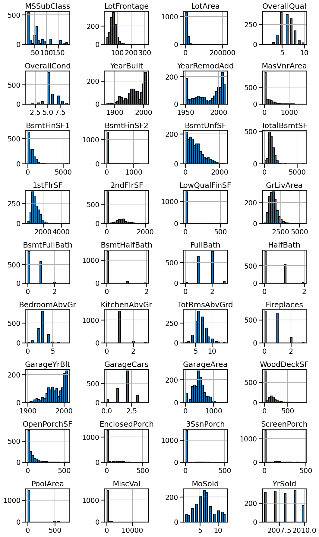
We see that some features have high picks for 0. It could be linked that this value was assigned when the criterion did not apply, for instance the area of the swimming pool when no swimming pools are available.
We also have some feature encoding some date (for instance year).
These information are useful and should also be considered when designing a predictive model.
Now, let’s have a look at the data encoded with strings.
string_data = data.select_dtypes(object)
string_data.info()
<class 'pandas.core.frame.DataFrame'>
RangeIndex: 1460 entries, 0 to 1459
Data columns (total 43 columns):
 #   Column         Non-Null Count  Dtype
---  ------         --------------  -----
 0   MSZoning       1460 non-null   object
 1   Street         1460 non-null   object
 2   Alley          91 non-null     object
 3   LotShape       1460 non-null   object
 4   LandContour    1460 non-null   object
 5   Utilities      1460 non-null   object
 6   LotConfig      1460 non-null   object
 7   LandSlope      1460 non-null   object
 8   Neighborhood   1460 non-null   object
 9   Condition1     1460 non-null   object
 10  Condition2     1460 non-null   object
 11  BldgType       1460 non-null   object
 12  HouseStyle     1460 non-null   object
 13  RoofStyle      1460 non-null   object
 14  RoofMatl       1460 non-null   object
 15  Exterior1st    1460 non-null   object
 16  Exterior2nd    1460 non-null   object
 17  MasVnrType     588 non-null    object
 18  ExterQual      1460 non-null   object
 19  ExterCond      1460 non-null   object
 20  Foundation     1460 non-null   object
 21  BsmtQual       1423 non-null   object
 22  BsmtCond       1423 non-null   object
 23  BsmtExposure   1422 non-null   object
 24  BsmtFinType1   1423 non-null   object
 25  BsmtFinType2   1422 non-null   object
 26  Heating        1460 non-null   object
 27  HeatingQC      1460 non-null   object
 28  CentralAir     1460 non-null   object
 29  Electrical     1459 non-null   object
 30  KitchenQual    1460 non-null   object
 31  Functional     1460 non-null   object
 32  FireplaceQu    770 non-null    object
 33  GarageType     1379 non-null   object
 34  GarageFinish   1379 non-null   object
 35  GarageQual     1379 non-null   object
 36  GarageCond     1379 non-null   object
 37  PavedDrive     1460 non-null   object
 38  PoolQC         7 non-null      object
 39  Fence          281 non-null    object
 40  MiscFeature    54 non-null     object
 41  SaleType       1460 non-null   object
 42  SaleCondition  1460 non-null   object
dtypes: object(43)
memory usage: 490.6+ KB
These features are categorical. We can make some bar plot to see categories count for each feature.
from math import ceil
from itertools import zip_longest

n_string_features = string_data.shape[1]
nrows, ncols = ceil(n_string_features / 4), 4

fig, axs = plt.subplots(ncols=ncols, nrows=nrows, figsize=(14, 80))

for feature_name, ax in zip_longest(string_data, axs.ravel()):
    if feature_name is None:
        # do not show the axis
        ax.axis("off")
        continue

    string_data[feature_name].value_counts().plot.barh(ax=ax)
    ax.set_title(feature_name)

plt.subplots_adjust(hspace=0.2, wspace=0.8)
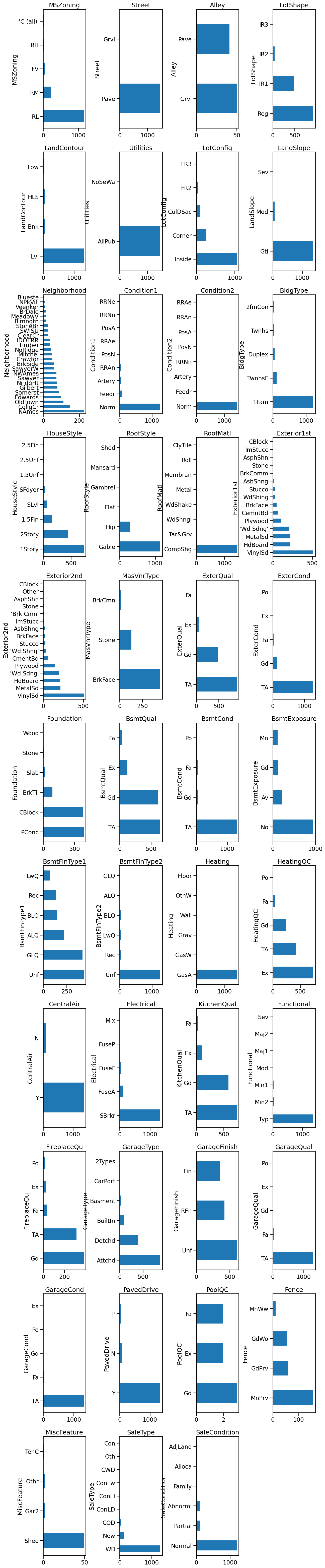
Plotting this information allows us to answer to two questions:
Is there few or many categories for a given features?
Is there rare categories for some features?
Knowing about these peculiarities would help at designing the predictive pipeline.
Note
In order to keep the content of the course simple and didactic, we created a version of this database without missing values.
ames_housing_no_missing = pd.read_csv(
    "../datasets/ames_housing_no_missing.csv"
)
ames_housing_no_missing.head()
| MSSubClass | MSZoning | LotFrontage | LotArea | Street | Alley | LotShape | LandContour | Utilities | LotConfig | ... | PoolArea | PoolQC | Fence | MiscFeature | MiscVal | MoSold | YrSold | SaleType | SaleCondition | SalePrice | |
|---|---|---|---|---|---|---|---|---|---|---|---|---|---|---|---|---|---|---|---|---|---|
| 0 | 60 | RL | 65.0 | 8450 | Pave | Grvl | Reg | Lvl | AllPub | Inside | ... | 0 | Gd | MnPrv | Shed | 0 | 2 | 2008 | WD | Normal | 208500 |
| 1 | 20 | RL | 80.0 | 9600 | Pave | Grvl | Reg | Lvl | AllPub | FR2 | ... | 0 | Gd | MnPrv | Shed | 0 | 5 | 2007 | WD | Normal | 181500 |
| 2 | 60 | RL | 68.0 | 11250 | Pave | Grvl | IR1 | Lvl | AllPub | Inside | ... | 0 | Gd | MnPrv | Shed | 0 | 9 | 2008 | WD | Normal | 223500 |
| 3 | 70 | RL | 60.0 | 9550 | Pave | Grvl | IR1 | Lvl | AllPub | Corner | ... | 0 | Gd | MnPrv | Shed | 0 | 2 | 2006 | WD | Abnorml | 140000 |
| 4 | 60 | RL | 84.0 | 14260 | Pave | Grvl | IR1 | Lvl | AllPub | FR2 | ... | 0 | Gd | MnPrv | Shed | 0 | 12 | 2008 | WD | Normal | 250000 |
5 rows × 80 columns
It contains the same information as the original dataset after using a
sklearn.impute.SimpleImputer
to replace missing values using the mean along each numerical column
(including the target), and the most frequent value along each categorical
column.
from sklearn.compose import make_column_transformer
from sklearn.impute import SimpleImputer
from sklearn.pipeline import make_pipeline

numerical_features = [
    "LotFrontage",
    "LotArea",
    "MasVnrArea",
    "BsmtFinSF1",
    "BsmtFinSF2",
    "BsmtUnfSF",
    "TotalBsmtSF",
    "1stFlrSF",
    "2ndFlrSF",
    "LowQualFinSF",
    "GrLivArea",
    "BedroomAbvGr",
    "KitchenAbvGr",
    "TotRmsAbvGrd",
    "Fireplaces",
    "GarageCars",
    "GarageArea",
    "WoodDeckSF",
    "OpenPorchSF",
    "EnclosedPorch",
    "3SsnPorch",
    "ScreenPorch",
    "PoolArea",
    "MiscVal",
    target_name,
]
categorical_features = data.columns.difference(numerical_features)

most_frequent_imputer = SimpleImputer(strategy="most_frequent")
mean_imputer = SimpleImputer(strategy="mean")

preprocessor = make_column_transformer(
    (most_frequent_imputer, categorical_features),
    (mean_imputer, numerical_features),
)
ames_housing_preprocessed = pd.DataFrame(
    preprocessor.fit_transform(ames_housing),
    columns=categorical_features.tolist() + numerical_features,
)
ames_housing_preprocessed = ames_housing_preprocessed[ames_housing.columns]
ames_housing_preprocessed = ames_housing_preprocessed.astype(
    ames_housing.dtypes
)
(ames_housing_no_missing == ames_housing_preprocessed).all()
MSSubClass       True
MSZoning         True
LotFrontage      True
LotArea          True
Street           True
                 ...
MoSold           True
YrSold           True
SaleType         True
SaleCondition    True
SalePrice        True
Length: 80, dtype: bool