Analysis of hyperparameter search results

In the previous notebook we showed how to implement a randomized search for tuning the hyperparameters of a HistGradientBoostingClassifier to fit the adult_census dataset. In practice, a randomized hyperparameter search is usually run with a large number of iterations.

In order to avoid the computational cost and still make a decent analysis, we load the results obtained from a similar search with 500 iterations.

import pandas as pd

cv_results = pd.read_csv(
    "../figures/randomized_search_results.csv", index_col=0
)
cv_results

	mean_fit_time	std_fit_time	mean_score_time	std_score_time	param_classifier__l2_regularization	param_classifier__learning_rate	param_classifier__max_bins	param_classifier__max_leaf_nodes	param_classifier__min_samples_leaf	params	split0_test_score	split1_test_score	split2_test_score	split3_test_score	split4_test_score	mean_test_score	std_test_score	rank_test_score
0	0.540456	0.062725	0.052069	0.002661	2.467047	0.550075	86	22	6	{'classifier__l2_regularization': 2.4670474863...	0.856558	0.862271	0.857767	0.854491	0.856675	0.857552	0.002586	48
1	1.110536	0.033403	0.074142	0.002165	0.015449	0.001146	60	19	1	{'classifier__l2_regularization': 0.0154488709...	0.758974	0.758941	0.758941	0.758941	0.758941	0.758947	0.000013	323
2	1.137484	0.053150	0.092993	0.029005	1.095093	0.004274	151	17	10	{'classifier__l2_regularization': 1.0950934559...	0.783267	0.758941	0.776413	0.779143	0.758941	0.771341	0.010357	311
3	3.935108	0.202993	0.118105	0.023658	0.003621	0.001305	18	164	37	{'classifier__l2_regularization': 0.0036210968...	0.758974	0.758941	0.758941	0.758941	0.758941	0.758947	0.000013	323
4	0.255219	0.038301	0.056048	0.016736	0.000081	5.407382	97	8	3	{'classifier__l2_regularization': 8.1060737427...	0.758974	0.758941	0.758941	0.758941	0.758941	0.758947	0.000013	323
...	...	...	...	...	...	...	...	...	...	...	...	...	...	...	...	...	...	...
495	0.452411	0.023006	0.055563	0.000846	0.000075	0.364373	92	17	4	{'classifier__l2_regularization': 7.4813767874...	0.858332	0.865001	0.862681	0.860360	0.860770	0.861429	0.002258	34
496	1.133042	0.014456	0.078186	0.002199	5.065946	0.001222	7	17	1	{'classifier__l2_regularization': 5.0659455480...	0.758974	0.758941	0.758941	0.758941	0.758941	0.758947	0.000013	323
497	0.911828	0.017167	0.076563	0.005130	2.460025	0.044408	16	7	7	{'classifier__l2_regularization': 2.4600250010...	0.839907	0.849713	0.846847	0.846028	0.844390	0.845377	0.003234	140
498	1.168120	0.121819	0.061283	0.000760	0.000068	0.287904	227	146	5	{'classifier__l2_regularization': 6.7755366885...	0.861881	0.865001	0.862408	0.859951	0.861862	0.862221	0.001623	33
499	0.823774	0.120686	0.060351	0.014958	0.445218	0.005112	19	8	19	{'classifier__l2_regularization': 0.4452178932...	0.764569	0.765902	0.765902	0.764947	0.765083	0.765281	0.000535	319

500 rows × 18 columns

We define a function to remove the prefixes in the hyperparameters column names.

def shorten_param(param_name):
    if "__" in param_name:
        return param_name.rsplit("__", 1)[1]
    return param_name


cv_results = cv_results.rename(shorten_param, axis=1)
cv_results

	mean_fit_time	std_fit_time	mean_score_time	std_score_time	l2_regularization	learning_rate	max_bins	max_leaf_nodes	min_samples_leaf	params	split0_test_score	split1_test_score	split2_test_score	split3_test_score	split4_test_score	mean_test_score	std_test_score	rank_test_score
0	0.540456	0.062725	0.052069	0.002661	2.467047	0.550075	86	22	6	{'classifier__l2_regularization': 2.4670474863...	0.856558	0.862271	0.857767	0.854491	0.856675	0.857552	0.002586	48
1	1.110536	0.033403	0.074142	0.002165	0.015449	0.001146	60	19	1	{'classifier__l2_regularization': 0.0154488709...	0.758974	0.758941	0.758941	0.758941	0.758941	0.758947	0.000013	323
2	1.137484	0.053150	0.092993	0.029005	1.095093	0.004274	151	17	10	{'classifier__l2_regularization': 1.0950934559...	0.783267	0.758941	0.776413	0.779143	0.758941	0.771341	0.010357	311
3	3.935108	0.202993	0.118105	0.023658	0.003621	0.001305	18	164	37	{'classifier__l2_regularization': 0.0036210968...	0.758974	0.758941	0.758941	0.758941	0.758941	0.758947	0.000013	323
4	0.255219	0.038301	0.056048	0.016736	0.000081	5.407382	97	8	3	{'classifier__l2_regularization': 8.1060737427...	0.758974	0.758941	0.758941	0.758941	0.758941	0.758947	0.000013	323
...	...	...	...	...	...	...	...	...	...	...	...	...	...	...	...	...	...	...
495	0.452411	0.023006	0.055563	0.000846	0.000075	0.364373	92	17	4	{'classifier__l2_regularization': 7.4813767874...	0.858332	0.865001	0.862681	0.860360	0.860770	0.861429	0.002258	34
496	1.133042	0.014456	0.078186	0.002199	5.065946	0.001222	7	17	1	{'classifier__l2_regularization': 5.0659455480...	0.758974	0.758941	0.758941	0.758941	0.758941	0.758947	0.000013	323
497	0.911828	0.017167	0.076563	0.005130	2.460025	0.044408	16	7	7	{'classifier__l2_regularization': 2.4600250010...	0.839907	0.849713	0.846847	0.846028	0.844390	0.845377	0.003234	140
498	1.168120	0.121819	0.061283	0.000760	0.000068	0.287904	227	146	5	{'classifier__l2_regularization': 6.7755366885...	0.861881	0.865001	0.862408	0.859951	0.861862	0.862221	0.001623	33
499	0.823774	0.120686	0.060351	0.014958	0.445218	0.005112	19	8	19	{'classifier__l2_regularization': 0.4452178932...	0.764569	0.765902	0.765902	0.764947	0.765083	0.765281	0.000535	319

500 rows × 18 columns

As we have more than 2 parameters in our randomized-search, we cannot visualize the results using a heatmap. We could still do it pair-wise, but having a two-dimensional projection of a multi-dimensional problem can lead to a wrong interpretation of the scores.

import seaborn as sns
import numpy as np

df = pd.DataFrame(
    {
        "max_leaf_nodes": cv_results["max_leaf_nodes"],
        "learning_rate": cv_results["learning_rate"],
        "score_bin": pd.cut(
            cv_results["mean_test_score"], bins=np.linspace(0.5, 1.0, 6)
        ),
    }
)
sns.set_palette("YlGnBu_r")
ax = sns.scatterplot(
    data=df,
    x="max_leaf_nodes",
    y="learning_rate",
    hue="score_bin",
    s=50,
    color="k",
    edgecolor=None,
)
ax.set_xscale("log")
ax.set_yscale("log")

_ = ax.legend(
    title="mean_test_score", loc="center left", bbox_to_anchor=(1, 0.5)
)

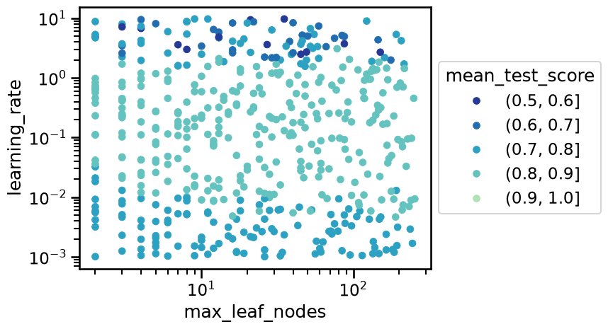
In the previous plot we see that the top performing values are located in a band of learning rate between 0.01 and 1.0, but we have no control in how the other hyperparameters interact with such values for the learning rate. Instead, we can visualize all the hyperparameters at the same time using a parallel coordinates plot.

import numpy as np
import plotly.express as px

fig = px.parallel_coordinates(
    cv_results.rename(shorten_param, axis=1).apply(
        {
            "learning_rate": np.log10,
            "max_leaf_nodes": np.log2,
            "max_bins": np.log2,
            "min_samples_leaf": np.log10,
            "l2_regularization": np.log10,
            "mean_test_score": lambda x: x,
        }
    ),
    color="mean_test_score",
    color_continuous_scale=px.colors.sequential.Viridis,
)
fig.show()

Note

We transformed most axis values by taking a log10 or log2 to spread the active ranges and improve the readability of the plot.

The parallel coordinates plot displays the values of the hyperparameters on different columns while the performance metric is color coded. Thus, we are able to quickly inspect if there is a range of hyperparameters which is working or not.

It is possible to select a range of results by clicking and holding on any axis of the parallel coordinate plot. You can then slide (move) the range selection and cross two selections to see the intersections. You can undo a selection by clicking once again on the same axis.

In particular for this hyperparameter search, it is interesting to confirm that the yellow lines (top performing models) all reach intermediate values for the learning rate, that is, tick values between -2 and 0 which correspond to learning rate values of 0.01 to 1.0 once we invert back the log10 transform for that axis.

But now we can also observe that it is not possible to select the highest performing models by selecting lines of on the max_bins axis with tick values between 1 and 3.

The other hyperparameters are not very sensitive. We can check that if we select the learning_rate axis tick values between -1.5 and -0.5 and max_bins tick values between 5 and 8, we always select top performing models, whatever the values of the other hyperparameters.

In this notebook, we saw how to interactively explore the results of a large randomized search with multiple interacting hyperparameters. In particular we observed that some hyperparameters have very little impact on the cross-validation score, while others have to be adjusted within a specific range to get models with good predictive accuracy.