Decision tree for regression

In this notebook, we present how decision trees are working in regression problems. We show differences with the decision trees previously presented in a classification setting.

First, we load the penguins dataset specifically for solving a regression problem.

Note

If you want a deeper overview regarding this dataset, you can refer to the Appendix - Datasets description section at the end of this MOOC.

import pandas as pd

penguins = pd.read_csv("../datasets/penguins_regression.csv")

feature_name = "Flipper Length (mm)"
target_name = "Body Mass (g)"
data_train, target_train = penguins[[feature_name]], penguins[target_name]

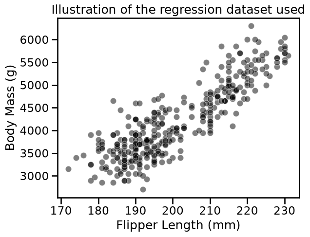
To illustrate how decision trees predict in a regression setting, we create a synthetic dataset containing some of the possible flipper length values between the minimum and the maximum of the original data.

import numpy as np

data_test = pd.DataFrame(
    np.arange(data_train[feature_name].min(), data_train[feature_name].max()),
    columns=[feature_name],
)

Using the term “test” here refers to data that was not used for training. It should not be confused with data coming from a train-test split, as it was generated in equally-spaced intervals for the visual evaluation of the predictions.

Note that this is methodologically valid here because our objective is to get some intuitive understanding on the shape of the decision function of the learned decision trees.

However, computing an evaluation metric on such a synthetic test set would be meaningless since the synthetic dataset does not follow the same distribution as the real world data on which the model would be deployed.

import matplotlib.pyplot as plt
import seaborn as sns

sns.scatterplot(
    data=penguins, x=feature_name, y=target_name, color="black", alpha=0.5
)
_ = plt.title("Illustration of the regression dataset used")

We first illustrate the difference between a linear model and a decision tree.

from sklearn.linear_model import LinearRegression

linear_model = LinearRegression()
linear_model.fit(data_train, target_train)
target_predicted = linear_model.predict(data_test)

sns.scatterplot(
    data=penguins, x=feature_name, y=target_name, color="black", alpha=0.5
)
plt.plot(data_test[feature_name], target_predicted, label="Linear regression")
plt.legend()
_ = plt.title("Prediction function using a LinearRegression")

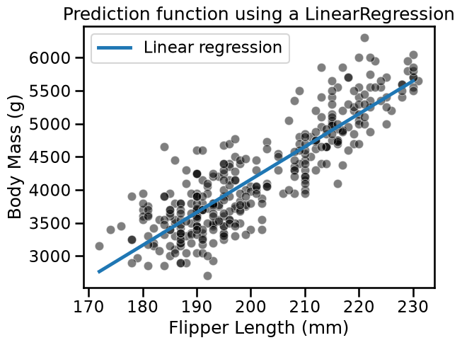
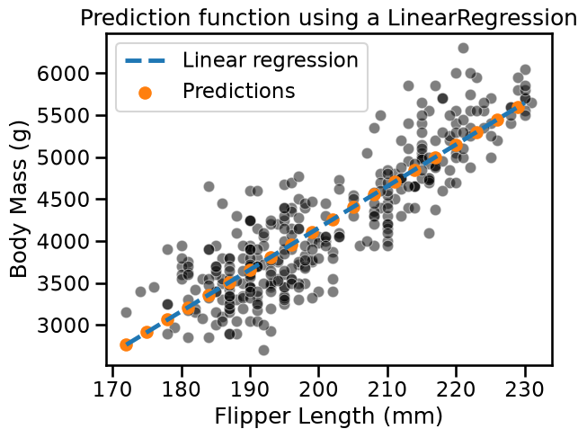
On the plot above, we see that a non-regularized LinearRegression is able to fit the data. A feature of this model is that all new predictions will be on the line.

ax = sns.scatterplot(
    data=penguins, x=feature_name, y=target_name, color="black", alpha=0.5
)
plt.plot(
    data_test[feature_name],
    target_predicted,
    label="Linear regression",
    linestyle="--",
)
plt.scatter(
    data_test[::3],
    target_predicted[::3],
    label="Predictions",
    color="tab:orange",
)
plt.legend()
_ = plt.title("Prediction function using a LinearRegression")

Contrary to linear models, decision trees are non-parametric models: they do not make assumptions about the way data is distributed. This affects the prediction scheme. Repeating the above experiment highlights the differences.

from sklearn.tree import DecisionTreeRegressor

tree = DecisionTreeRegressor(max_depth=1)
tree.fit(data_train, target_train)
target_predicted = tree.predict(data_test)

sns.scatterplot(
    data=penguins, x=feature_name, y=target_name, color="black", alpha=0.5
)
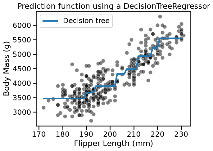
plt.plot(data_test[feature_name], target_predicted, label="Decision tree")
plt.legend()
_ = plt.title("Prediction function using a DecisionTreeRegressor")

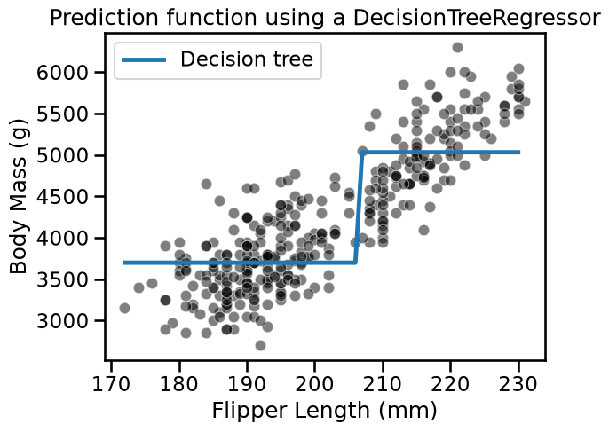
We see that the decision tree model does not have an a priori distribution for the data and we do not end-up with a straight line to regress flipper length and body mass.

Instead, we observe that the predictions of the tree are piecewise constant. Indeed, our feature space was split into two partitions. Let’s check the tree structure to see what was the threshold found during the training.

from sklearn.tree import plot_tree

_, ax = plt.subplots(figsize=(8, 6))
_ = plot_tree(tree, feature_names=[feature_name], ax=ax)

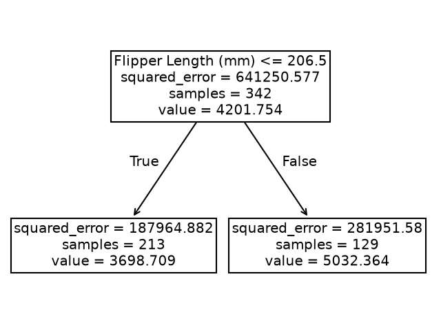
The threshold for our feature (flipper length) is 206.5 mm. The predicted values on each side of the split are two constants: 3698.71 g and 5032.36 g. These values corresponds to the mean values of the training samples in each partition.

In classification, we saw that increasing the depth of the tree allowed us to get more complex decision boundaries. Let’s check the effect of increasing the depth in a regression setting:

tree = DecisionTreeRegressor(max_depth=3)
tree.fit(data_train, target_train)
target_predicted = tree.predict(data_test)

sns.scatterplot(
    data=penguins, x=feature_name, y=target_name, color="black", alpha=0.5
)
plt.plot(data_test[feature_name], target_predicted, label="Decision tree")
plt.legend()
_ = plt.title("Prediction function using a DecisionTreeRegressor")

Increasing the depth of the tree increases the number of partitions and thus the number of constant values that the tree is capable of predicting.

In this notebook, we highlighted the differences in behavior of a decision tree used in a classification problem in contrast to a regression problem.