📃 Solution for Exercise M6.02

The aim of this exercise it to explore some attributes available in scikit-learn’s random forest.

First, we will fit the penguins regression dataset.

import pandas as pd
from sklearn.model_selection import train_test_split

penguins = pd.read_csv("../datasets/penguins_regression.csv")
feature_name = "Flipper Length (mm)"
target_name = "Body Mass (g)"
data, target = penguins[[feature_name]], penguins[target_name]
data_train, data_test, target_train, target_test = train_test_split(
    data, target, random_state=0
)

Note

If you want a deeper overview regarding this dataset, you can refer to the Appendix - Datasets description section at the end of this MOOC.

Create a random forest containing three trees. Train the forest and check the generalization performance on the testing set in terms of mean absolute error.

# solution
from sklearn.metrics import mean_absolute_error
from sklearn.ensemble import RandomForestRegressor

forest = RandomForestRegressor(n_estimators=3)
forest.fit(data_train, target_train)
target_predicted = forest.predict(data_test)
print(
    "Mean absolute error: "
    f"{mean_absolute_error(target_test, target_predicted):.3f} grams"
)

Mean absolute error: 355.129 grams

We now aim to plot the predictions from the individual trees in the forest. For that purpose you have to create first a new dataset containing evenly spaced values for the flipper length over the interval between 170 mm and 230 mm.

# solution
import numpy as np

data_range = pd.DataFrame(np.linspace(170, 235, num=300), columns=data.columns)

The trees contained in the forest that you created can be accessed with the attribute estimators_. Use them to predict the body mass corresponding to the values in this newly created dataset. Similarly find the predictions of the random forest in this dataset.

# solution
tree_predictions = []

for tree in forest.estimators_:
    # we convert `data_range` into a NumPy array to avoid a warning raised in scikit-learn
    tree_predictions.append(tree.predict(data_range.to_numpy()))

forest_predictions = forest.predict(data_range)

Now make a plot that displays:

• the whole data using a scatter plot;

• the decision of each individual tree;

• the decision of the random forest.

# solution
import matplotlib.pyplot as plt
import seaborn as sns

sns.scatterplot(
    data=penguins, x=feature_name, y=target_name, color="black", alpha=0.5
)

# plot tree predictions
for tree_idx, predictions in enumerate(tree_predictions):
    plt.plot(
        data_range[feature_name],
        predictions,
        label=f"Tree #{tree_idx}",
        linestyle="--",
        alpha=0.8,
    )

plt.plot(data_range[feature_name], forest_predictions, label="Random forest")
_ = plt.legend(bbox_to_anchor=(1.05, 0.8), loc="upper left")

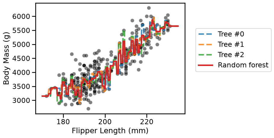
The random forest reduces the overfitting of the individual trees but still overfits itself. In the section on “hyperparameter tuning with ensemble methods” we will see how to further mitigate this effect. Still, interested users may increase the number of estimators in the forest and try different values of, e.g., min_samples_split.