Regularization of linear regression model

In this notebook, we explore some limitations of linear regression models and demonstrate the benefits of using regularized models instead. Additionally, we discuss the importance of scaling the data when working with regularized models, especially when tuning the regularization parameter.

We start by highlighting the problem of overfitting that can occur with a simple linear regression model.

Effect of regularization

We load the Ames housing dataset. We retain some specific features_of_interest.

Note

If you want a deeper overview regarding this dataset, you can refer to the Appendix - Datasets description section at the end of this MOOC.

import pandas as pd

ames_housing = pd.read_csv("../datasets/ames_housing_no_missing.csv")
features_of_interest = [
    "LotFrontage",
    "LotArea",
    "PoolArea",
    "YearBuilt",
    "YrSold",
]
target_name = "SalePrice"
data, target = (
    ames_housing[features_of_interest],
    ames_housing[target_name],
)

In one of the previous notebooks, we showed that linear models could be used even when there is no linear relationship between the data and target. For instance, one can use the PolynomialFeatures transformer to create additional features that capture some non-linear interactions between them.

Here, we use this transformer to augment the feature space. Subsequently, we train a linear regression model. We use cross-validation with return_train_score=True to evaluate both the train scores and the generalization capabilities of our model.

from sklearn.model_selection import cross_validate
from sklearn.pipeline import make_pipeline
from sklearn.preprocessing import PolynomialFeatures
from sklearn.linear_model import LinearRegression

linear_regression = make_pipeline(
    PolynomialFeatures(degree=2, include_bias=False), LinearRegression()
).set_output(transform="pandas")
cv_results = cross_validate(
    linear_regression,
    data,
    target,
    cv=10,
    scoring="neg_mean_squared_error",
    return_train_score=True,
    return_estimator=True,
)

We can compare the mean squared error on the training and testing set to assess the generalization performance of our model.

train_error = -cv_results["train_score"]
print(
    "Mean squared error of linear regression model on the train set:\n"
    f"{train_error.mean():.2e} ± {train_error.std():.2e}"
)

Mean squared error of linear regression model on the train set:
2.85e+09 ± 8.63e+07

test_error = -cv_results["test_score"]
print(
    "Mean squared error of linear regression model on the test set:\n"
    f"{test_error.mean():.2e} ± {test_error.std():.2e}"
)

Mean squared error of linear regression model on the test set:
8.69e+10 ± 2.47e+11

The training error is in average one order of magnitude lower than the testing error (lower error is better). Such a gap between the training and testing scores is an indication that our model overfitted the training set. Indeed, this is one of the dangers when augmenting the number of features with a PolynomialFeatures transformer. For instance, one does not expect features such as PoolArea * YrSold to be very predictive.

To analyze the weights of the model, we can create a dataframe. The columns of the dataframe contain the feature names, while the rows store the coefficients of each model of a given cross-validation fold.

In order to obtain the feature names associated with each feature combination, we need to extract them from the augmented data created by PolynomialFeatures. Fortunately, scikit-learn provides a convenient method called feature_names_in_ for this purpose. Let’s begin by retrieving the coefficients from the model fitted in the first cross-validation fold.

model_first_fold = cv_results["estimator"][0]
model_first_fold

Pipeline(steps=[('polynomialfeatures', PolynomialFeatures(include_bias=False)),
                ('linearregression', LinearRegression())])

In a Jupyter environment, please rerun this cell to show the HTML representation or trust the notebook.
On GitHub, the HTML representation is unable to render, please try loading this page with nbviewer.org.

Now, we can access the fitted LinearRegression (step -1 i.e. the last step of the linear_regression pipeline) to recover the feature names.

feature_names = model_first_fold[-1].feature_names_in_
feature_names

array(['LotFrontage', 'LotArea', 'PoolArea', 'YearBuilt', 'YrSold',
       'LotFrontage^2', 'LotFrontage LotArea', 'LotFrontage PoolArea',
       'LotFrontage YearBuilt', 'LotFrontage YrSold', 'LotArea^2',
       'LotArea PoolArea', 'LotArea YearBuilt', 'LotArea YrSold',
       'PoolArea^2', 'PoolArea YearBuilt', 'PoolArea YrSold',
       'YearBuilt^2', 'YearBuilt YrSold', 'YrSold^2'], dtype=object)

The following code creates a list by iterating through the estimators and querying their last step for the learned coef_. We can then create the dataframe containing all the information.

import pandas as pd

coefs = [est[-1].coef_ for est in cv_results["estimator"]]
weights_linear_regression = pd.DataFrame(coefs, columns=feature_names)

Now, let’s use a box plot to see the coefficients variations.

import matplotlib.pyplot as plt

color = {"whiskers": "black", "medians": "black", "caps": "black"}
fig, ax = plt.subplots(figsize=(10, 10))
weights_linear_regression.plot.box(color=color, vert=False, ax=ax)
_ = ax.set(title="Linear regression weights (linear scale)")

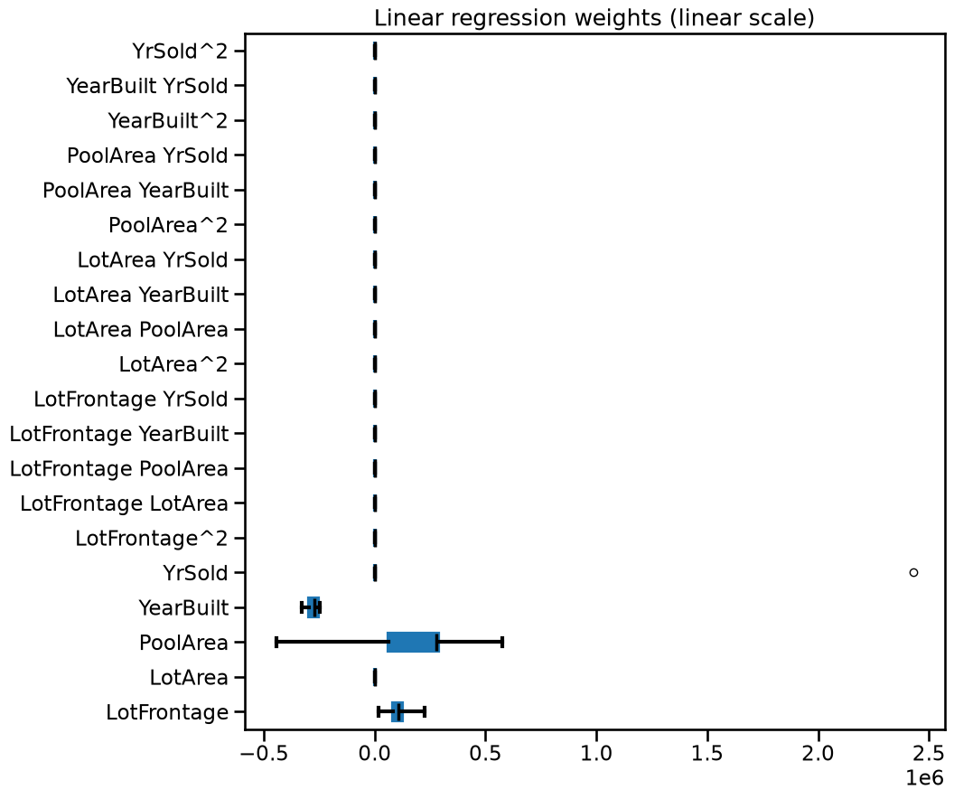
By looking at the bar plot above it would seem that most of the features are very close to zero, but this is just an effect of visualizing them on the same scale as the extremely large span of "YrSold". Instead we can use a symmetric log scale for the plot.

color = {"whiskers": "black", "medians": "black", "caps": "black"}
fig, ax = plt.subplots(figsize=(10, 10))
weights_linear_regression.plot.box(color=color, vert=False, ax=ax)
_ = ax.set(
    title="Linear regression weights (symmetric log scale)",
    xscale="symlog",
)

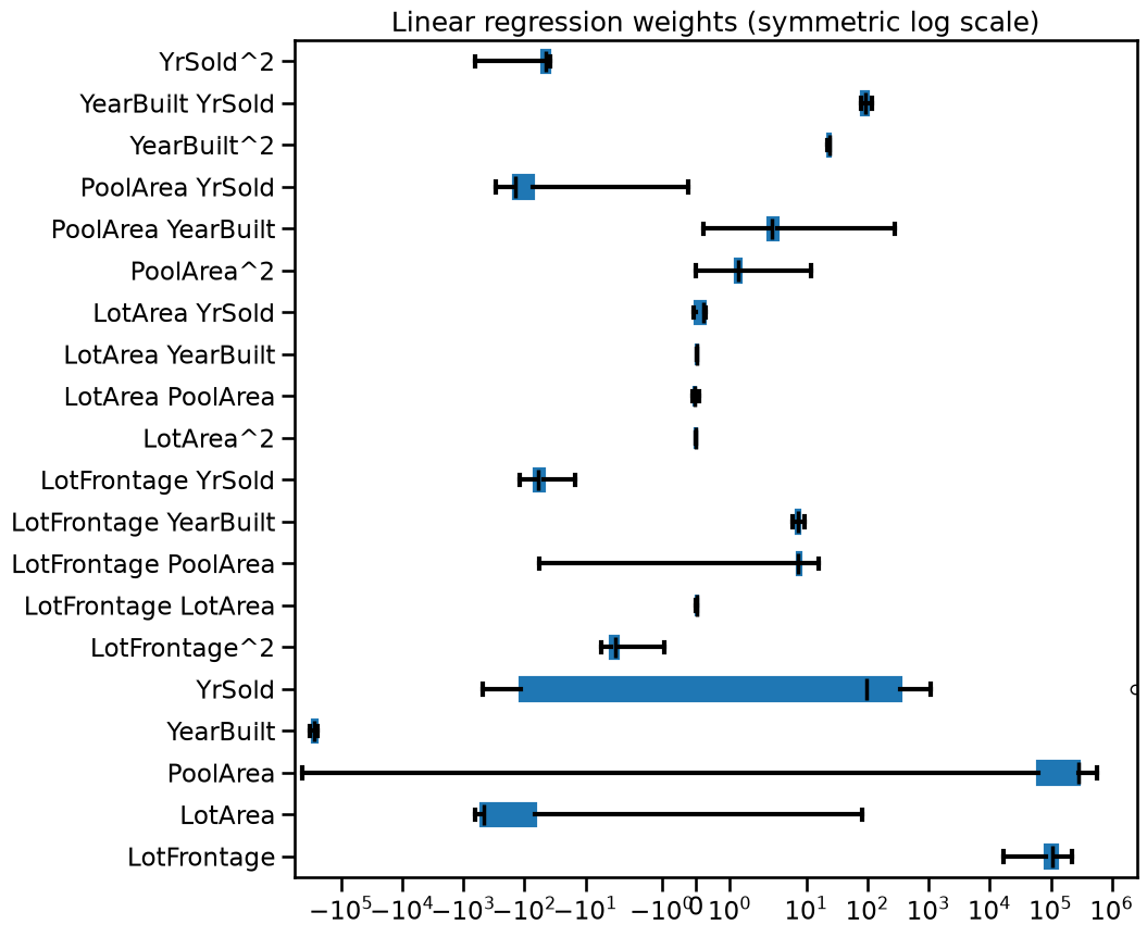
Observe that some coefficients are extremely large while others are extremely small, yet non-zero. Furthermore, the coefficient values can be very unstable across cross-validation folds.

We can force the linear regression model to consider all features in a more homogeneous manner. In fact, we could force large positive or negative weights to shrink toward zero. This is known as regularization. We use a ridge model which enforces such behavior.

from sklearn.linear_model import Ridge

ridge = make_pipeline(
    PolynomialFeatures(degree=2, include_bias=False),
    Ridge(alpha=100, solver="cholesky"),
)
cv_results = cross_validate(
    ridge,
    data,
    target,
    cv=20,
    scoring="neg_mean_squared_error",
    return_train_score=True,
    return_estimator=True,
)

/opt/hostedtoolcache/Python/3.9.18/x64/lib/python3.9/site-packages/sklearn/linear_model/_ridge.py:204: LinAlgWarning: Ill-conditioned matrix (rcond=2.59923e-20): result may not be accurate.
  return linalg.solve(A, Xy, assume_a="pos", overwrite_a=True).T
/opt/hostedtoolcache/Python/3.9.18/x64/lib/python3.9/site-packages/sklearn/linear_model/_ridge.py:204: LinAlgWarning: Ill-conditioned matrix (rcond=2.59556e-20): result may not be accurate.
  return linalg.solve(A, Xy, assume_a="pos", overwrite_a=True).T
/opt/hostedtoolcache/Python/3.9.18/x64/lib/python3.9/site-packages/sklearn/linear_model/_ridge.py:204: LinAlgWarning: Ill-conditioned matrix (rcond=2.59609e-20): result may not be accurate.
  return linalg.solve(A, Xy, assume_a="pos", overwrite_a=True).T
/opt/hostedtoolcache/Python/3.9.18/x64/lib/python3.9/site-packages/sklearn/linear_model/_ridge.py:204: LinAlgWarning: Ill-conditioned matrix (rcond=3.11828e-20): result may not be accurate.
  return linalg.solve(A, Xy, assume_a="pos", overwrite_a=True).T
/opt/hostedtoolcache/Python/3.9.18/x64/lib/python3.9/site-packages/sklearn/linear_model/_ridge.py:204: LinAlgWarning: Ill-conditioned matrix (rcond=1.06109e-19): result may not be accurate.
  return linalg.solve(A, Xy, assume_a="pos", overwrite_a=True).T
/opt/hostedtoolcache/Python/3.9.18/x64/lib/python3.9/site-packages/sklearn/linear_model/_ridge.py:204: LinAlgWarning: Ill-conditioned matrix (rcond=2.60121e-20): result may not be accurate.
  return linalg.solve(A, Xy, assume_a="pos", overwrite_a=True).T
/opt/hostedtoolcache/Python/3.9.18/x64/lib/python3.9/site-packages/sklearn/linear_model/_ridge.py:204: LinAlgWarning: Ill-conditioned matrix (rcond=2.61694e-20): result may not be accurate.
  return linalg.solve(A, Xy, assume_a="pos", overwrite_a=True).T
/opt/hostedtoolcache/Python/3.9.18/x64/lib/python3.9/site-packages/sklearn/linear_model/_ridge.py:204: LinAlgWarning: Ill-conditioned matrix (rcond=2.59735e-20): result may not be accurate.
  return linalg.solve(A, Xy, assume_a="pos", overwrite_a=True).T
/opt/hostedtoolcache/Python/3.9.18/x64/lib/python3.9/site-packages/sklearn/linear_model/_ridge.py:204: LinAlgWarning: Ill-conditioned matrix (rcond=2.59566e-20): result may not be accurate.
  return linalg.solve(A, Xy, assume_a="pos", overwrite_a=True).T
/opt/hostedtoolcache/Python/3.9.18/x64/lib/python3.9/site-packages/sklearn/linear_model/_ridge.py:204: LinAlgWarning: Ill-conditioned matrix (rcond=2.72304e-20): result may not be accurate.
  return linalg.solve(A, Xy, assume_a="pos", overwrite_a=True).T
/opt/hostedtoolcache/Python/3.9.18/x64/lib/python3.9/site-packages/sklearn/linear_model/_ridge.py:204: LinAlgWarning: Ill-conditioned matrix (rcond=2.60047e-20): result may not be accurate.
  return linalg.solve(A, Xy, assume_a="pos", overwrite_a=True).T
/opt/hostedtoolcache/Python/3.9.18/x64/lib/python3.9/site-packages/sklearn/linear_model/_ridge.py:204: LinAlgWarning: Ill-conditioned matrix (rcond=2.59824e-20): result may not be accurate.
  return linalg.solve(A, Xy, assume_a="pos", overwrite_a=True).T
/opt/hostedtoolcache/Python/3.9.18/x64/lib/python3.9/site-packages/sklearn/linear_model/_ridge.py:204: LinAlgWarning: Ill-conditioned matrix (rcond=2.59593e-20): result may not be accurate.
  return linalg.solve(A, Xy, assume_a="pos", overwrite_a=True).T
/opt/hostedtoolcache/Python/3.9.18/x64/lib/python3.9/site-packages/sklearn/linear_model/_ridge.py:204: LinAlgWarning: Ill-conditioned matrix (rcond=2.59564e-20): result may not be accurate.
  return linalg.solve(A, Xy, assume_a="pos", overwrite_a=True).T
/opt/hostedtoolcache/Python/3.9.18/x64/lib/python3.9/site-packages/sklearn/linear_model/_ridge.py:204: LinAlgWarning: Ill-conditioned matrix (rcond=2.5959e-20): result may not be accurate.
  return linalg.solve(A, Xy, assume_a="pos", overwrite_a=True).T
/opt/hostedtoolcache/Python/3.9.18/x64/lib/python3.9/site-packages/sklearn/linear_model/_ridge.py:204: LinAlgWarning: Ill-conditioned matrix (rcond=2.59553e-20): result may not be accurate.
  return linalg.solve(A, Xy, assume_a="pos", overwrite_a=True).T
/opt/hostedtoolcache/Python/3.9.18/x64/lib/python3.9/site-packages/sklearn/linear_model/_ridge.py:204: LinAlgWarning: Ill-conditioned matrix (rcond=2.59686e-20): result may not be accurate.
  return linalg.solve(A, Xy, assume_a="pos", overwrite_a=True).T
/opt/hostedtoolcache/Python/3.9.18/x64/lib/python3.9/site-packages/sklearn/linear_model/_ridge.py:204: LinAlgWarning: Ill-conditioned matrix (rcond=2.60737e-20): result may not be accurate.
  return linalg.solve(A, Xy, assume_a="pos", overwrite_a=True).T
/opt/hostedtoolcache/Python/3.9.18/x64/lib/python3.9/site-packages/sklearn/linear_model/_ridge.py:204: LinAlgWarning: Ill-conditioned matrix (rcond=2.5957e-20): result may not be accurate.
  return linalg.solve(A, Xy, assume_a="pos", overwrite_a=True).T
/opt/hostedtoolcache/Python/3.9.18/x64/lib/python3.9/site-packages/sklearn/linear_model/_ridge.py:204: LinAlgWarning: Ill-conditioned matrix (rcond=2.60243e-20): result may not be accurate.
  return linalg.solve(A, Xy, assume_a="pos", overwrite_a=True).T

The code cell above can generate a couple of warnings (depending on the choice of solver) because the features included both extremely large and extremely small values, which are causing numerical problems when training the predictive model. We will get to that in a bit.

Let us evaluate the train and test scores of this model.

train_error = -cv_results["train_score"]
print(
    "Mean squared error of ridge model on the train set:\n"
    f"{train_error.mean():.2e} ± {train_error.std():.2e}"
)

Mean squared error of ridge model on the train set:
2.90e+09 ± 6.56e+07

test_error = -cv_results["test_score"]
print(
    "Mean squared error of ridge model on the test set:\n"
    f"{test_error.mean():.2e} ± {test_error.std():.2e}"
)

Mean squared error of ridge model on the test set:
4.55e+10 ± 1.68e+11

We see that the training and testing scores get closer, indicating that our model is less overfitting (yet still overfitting!). We can compare the values of the weights of ridge with the un-regularized linear regression.

coefs = [est[-1].coef_ for est in cv_results["estimator"]]
weights_ridge = pd.DataFrame(coefs, columns=feature_names)

fig, ax = plt.subplots(figsize=(8, 10))
weights_ridge.plot.box(color=color, vert=False, ax=ax)
_ = ax.set(title="Ridge regression weights")

Notice that the overall magnitudes of the weights are shrunk (yet non-zero!) with respect to the linear regression model. If you want to, feel free to use a symmetric log scale in the previous plot.

You can also observe that even if the weights’ values are less extreme, they are still unstable from one fold to another. Even worst, the results can vary a lot depending on the choice of the solver (for instance try to set solver="saga" or solver="lsqr" instead of solver="cholesky" and re-run the above cells).

In the following we attempt to resolve those remaining problems, by focusing on two important aspects we omitted so far:

• the need to scale the data, and

• the need to search for the best regularization parameter.

Feature scaling and regularization

On the one hand, weights define the association between feature values and the predicted target, which depends on the scales of both the feature values and the target. On the other hand, regularization adds constraints on the weights of the model through the alpha parameter. Therefore, the effect that feature rescaling has on the final weights also interacts with the use of regularization.

Let’s consider the case where features live on the same scale/units: if two features are found to be equally important by the model, they are affected similarly by the regularization strength.

Now, let’s consider the scenario where two features have completely different data scales (for instance age in years and annual revenue in dollars). Let’s also assume that both features are approximately equally predictive and are not too correlated. Fitting a linear regression without scaling and without regularization would give a higher weight to the feature with the smallest natural scale. If we add regularization, the feature with the smallest natural scale would be penalized more than the other feature. This is not desirable given the hypothesis that both features are equally important. In such case we require the regularization to stay neutral.

In practice, we don’t know ahead of time which features are predictive, and therefore we want regularization to treat all features approximately equally by default. This can be achieved by rescaling the features.

Furthermore, many numerical solvers used internally in scikit-learn behave better when features are approximately on the same scale. Heterogeneously scaled data can be detrimental when solving for the optimal weights (hence the warnings we tend to get when fitting linear models on raw data). Therefore, when working with a linear model and numerical data, it is generally a good practice to scale the data.

Thus, we add a MinMaxScaler in the machine learning pipeline, which scales each feature individually such that its range maps into the range between zero and one. We place it just before the PolynomialFeatures transformer as powers of features in the range between zero and one remain in the same range.

from sklearn.preprocessing import MinMaxScaler

scaled_ridge = make_pipeline(
    MinMaxScaler(),
    PolynomialFeatures(degree=2, include_bias=False),
    Ridge(alpha=10, solver="cholesky"),
)
cv_results = cross_validate(
    scaled_ridge,
    data,
    target,
    cv=10,
    scoring="neg_mean_squared_error",
    return_train_score=True,
    return_estimator=True,
)

train_error = -cv_results["train_score"]
print(
    "Mean squared error of scaled ridge model on the train set:\n"
    f"{train_error.mean():.2e} ± {train_error.std():.2e}"
)

Mean squared error of scaled ridge model on the train set:
3.78e+09 ± 1.21e+08

test_error = -cv_results["test_score"]
print(
    "Mean squared error of scaled ridge model on the test set:\n"
    f"{test_error.mean():.2e} ± {test_error.std():.2e}"
)

Mean squared error of scaled ridge model on the test set:
3.83e+09 ± 1.17e+09

We observe that scaling data has a positive impact on the test error: it is now both lower and closer to the train error. It means that our model is less overfitted and that we are getting closer to the best generalization sweet spot.

If you want to try different solvers, you can notice that fitting this pipeline no longer generates any warning regardless of such choice. Additionally, changing the solver should no longer result in significant changes in the weights.

Let’s have an additional look to the different weights.

coefs = [est[-1].coef_ for est in cv_results["estimator"]]
weights_ridge_scaled_data = pd.DataFrame(coefs, columns=feature_names)

fig, ax = plt.subplots(figsize=(8, 10))
weights_ridge_scaled_data.plot.box(color=color, vert=False, ax=ax)
_ = ax.set(title="Ridge regression weights with data scaling")

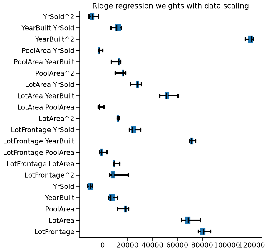
Compared to the previous plots, we see that now most weight magnitudes have a similar order of magnitude, i.e. they are more equally contributing. The number of unstable weights also decreased.

In the previous model, we set alpha=10. We can now check the impact of alpha by increasing it to a very large value.

ridge_large_alpha = make_pipeline(
    MinMaxScaler(),
    PolynomialFeatures(degree=2, include_bias=False),
    Ridge(alpha=1_000_000, solver="lsqr"),
)
cv_results = cross_validate(
    ridge_large_alpha,
    data,
    target,
    cv=10,
    scoring="neg_mean_squared_error",
    return_train_score=True,
    return_estimator=True,
)

coefs = [est[-1].coef_ for est in cv_results["estimator"]]
weights_ridge_scaled_data = pd.DataFrame(coefs, columns=feature_names)

fig, ax = plt.subplots(figsize=(8, 10))
weights_ridge_scaled_data.plot.box(color=color, vert=False, ax=ax)
_ = ax.set(title="Ridge regression weights with data scaling and large alpha")

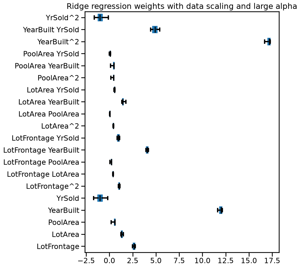
When examining the weight values, we notice that as the alpha value increases, the weights decrease. A negative value of alpha can lead to unpredictable and unstable behavior in the model.

Note

Here, we only focus on numerical features. For categorical features, it is generally common to omit scaling when features are encoded with a OneHotEncoder since the feature values are already on a similar scale.

However, this choice may depend on the scaling method and the user case. For instance, standard scaling categorical features that are imbalanced (e.g. more occurrences of a specific category) would even out the impact of regularization to each category. However, scaling such features in the presence of rare categories could be problematic (i.e. division by a very small standard deviation) and it can therefore introduce numerical issues.

In the previous analysis, we chose the parameter beforehand and fixed it for the analysis. In the next section, we check how the regularization parameter alpha should be tuned.

Tuning the regularization parameter

As mentioned, the regularization parameter needs to be tuned on each dataset. The default parameter does not lead to the optimal model. Therefore, we need to tune the alpha parameter.

Model hyperparameter tuning should be done with care. Indeed, we want to find an optimal parameter that maximizes some metrics. Thus, it requires both a training set and testing set.

However, this testing set should be different from the out-of-sample testing set that we used to evaluate our model: if we use the same one, we are using an alpha which was optimized for this testing set and it breaks the out-of-sample rule.

Therefore, we should include search of the hyperparameter alpha within the cross-validation. As we saw in previous notebooks, we could use a grid-search. However, some predictor in scikit-learn are available with an integrated hyperparameter search, more efficient than using a grid-search. The name of these predictors finishes by CV. In the case of Ridge, scikit-learn provides a RidgeCV regressor.

Cross-validating a pipeline that contains such predictors allows to make a nested cross-validation: the inner cross-validation searches for the best alpha, while the outer cross-validation gives an estimate of the testing score.

import numpy as np
from sklearn.linear_model import RidgeCV

alphas = np.logspace(-7, 5, num=100)
ridge = make_pipeline(
    MinMaxScaler(),
    PolynomialFeatures(degree=2, include_bias=False),
    RidgeCV(alphas=alphas, store_cv_values=True),
)

from sklearn.model_selection import ShuffleSplit

cv = ShuffleSplit(n_splits=50, random_state=0)
cv_results = cross_validate(
    ridge,
    data,
    target,
    cv=cv,
    scoring="neg_mean_squared_error",
    return_train_score=True,
    return_estimator=True,
    n_jobs=2,
)

train_error = -cv_results["train_score"]
print(
    "Mean squared error of tuned ridge model on the train set:\n"
    f"{train_error.mean():.2e} ± {train_error.std():.2e}"
)

Mean squared error of tuned ridge model on the train set:
3.12e+09 ± 1.25e+08

test_error = -cv_results["test_score"]
print(
    "Mean squared error of tuned ridge model on the test set:\n"
    f"{test_error.mean():.2e} ± {test_error.std():.2e}"
)

Mean squared error of tuned ridge model on the test set:
3.50e+09 ± 1.40e+09

By optimizing alpha, we see that the training and testing scores are close. It indicates that our model is not overfitting.

When fitting the ridge regressor, we also requested to store the error found during cross-validation (by setting the parameter store_cv_values=True). We can plot the mean squared error for the different alphas regularization strengths that we tried. The error bars represent one standard deviation of the average mean square error across folds for a given value of alpha.

mse_alphas = [
    est[-1].cv_values_.mean(axis=0) for est in cv_results["estimator"]
]
cv_alphas = pd.DataFrame(mse_alphas, columns=alphas)
cv_alphas = cv_alphas.aggregate(["mean", "std"]).T
cv_alphas

	mean	std
1.000000e-07	5.841881e+10	5.347783e+10
1.321941e-07	5.837563e+10	5.343115e+10
1.747528e-07	5.831866e+10	5.336956e+10
2.310130e-07	5.824352e+10	5.328835e+10
3.053856e-07	5.814452e+10	5.318133e+10
...	...	...
3.274549e+04	6.319038e+09	1.337394e+08
4.328761e+04	6.324503e+09	1.338181e+08
5.722368e+04	6.328652e+09	1.338778e+08
7.564633e+04	6.331799e+09	1.339232e+08
1.000000e+05	6.334185e+09	1.339576e+08

100 rows × 2 columns

fig, ax = plt.subplots(figsize=(8, 6))
ax.errorbar(cv_alphas.index, cv_alphas["mean"], yerr=cv_alphas["std"])
_ = ax.set(
    xscale="log",
    xlabel="alpha",
    yscale="log",
    ylabel="Mean squared error\n (lower is better)",
    title="Testing error in RidgeCV's inner cross-validation",
)

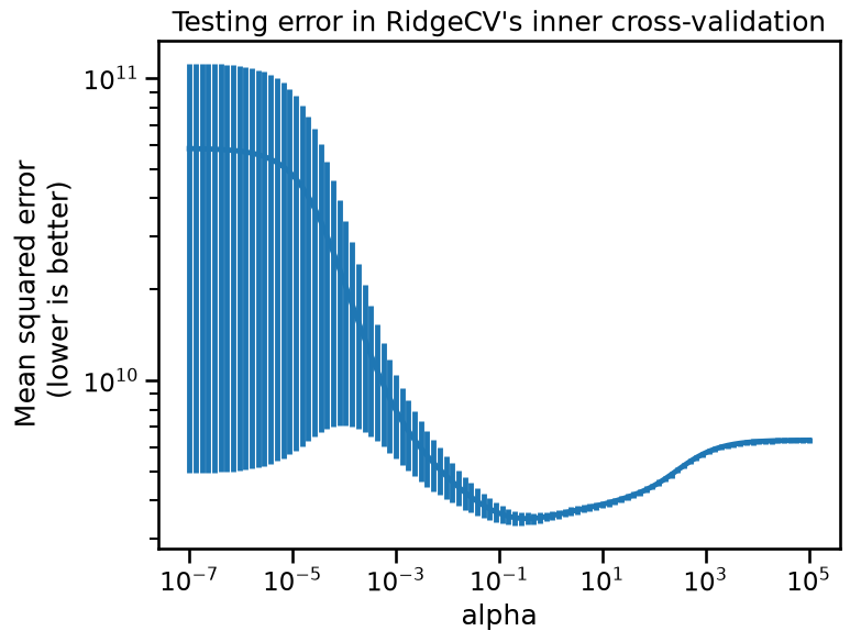
As we can see, regularization is just like salt in cooking: one must balance its amount to get the best generalization performance. We can check if the best alpha found is stable across the cross-validation fold.

best_alphas = [est[-1].alpha_ for est in cv_results["estimator"]]
best_alphas

[0.11497569953977356,
 0.35111917342151344,
 0.1519911082952933,
 0.35111917342151344,
 0.11497569953977356,
 0.4641588833612782,
 0.4641588833612782,
 0.4641588833612782,
 0.4641588833612782,
 0.35111917342151344,
 0.35111917342151344,
 0.4641588833612782,
 0.11497569953977356,
 0.11497569953977356,
 0.35111917342151344,
 0.4641588833612782,
 0.11497569953977356,
 0.35111917342151344,
 0.35111917342151344,
 0.35111917342151344,
 0.35111917342151344,
 0.4641588833612782,
 0.35111917342151344,
 0.4641588833612782,
 0.35111917342151344,
 0.35111917342151344,
 0.35111917342151344,
 0.08697490026177834,
 0.6135907273413176,
 0.4641588833612782,
 0.35111917342151344,
 0.4641588833612782,
 0.4641588833612782,
 0.11497569953977356,
 0.35111917342151344,
 0.35111917342151344,
 0.4641588833612782,
 0.35111917342151344,
 0.11497569953977356,
 0.08697490026177834,
 0.4641588833612782,
 0.4641588833612782,
 0.35111917342151344,
 0.35111917342151344,
 0.4641588833612782,
 0.35111917342151344,
 0.35111917342151344,
 0.35111917342151344,
 0.4641588833612782,
 0.35111917342151344]

The optimal regularization strength is not necessarily the same on all cross-validation iterations. But since we expect each cross-validation resampling to stem from the same data distribution, it is common practice to choose the best alpha to put into production as lying in the range defined by:

print(
    f"Min optimal alpha: {np.min(best_alphas):.2f} and "
    f"Max optimal alpha: {np.max(best_alphas):.2f}"
)

Min optimal alpha: 0.09 and Max optimal alpha: 0.61

This range can be reduced depending on the feature engineering and preprocessing.

Here is a summary of important points highlighted in this notebook:

• scaling features makes the effect of regularization more even: all variables are regularized by comparable magnitude, which would not necessarily be the case with the natural feature scales;

• scaling features makes the numerical solvers more stable which is also helpful to tune the regularization parameter more independently of the choice of the solver used to fit the linear model;

• tuning the regularization parameter of the Ridge estimator can be done very efficiently by using the RidgeCV class. Wrapping it into a cross_validate call makes it possible to assess the true generalization power of the whole pipeline by including the tuning of the regularization parameter as part of the learning process: this is an example of “nested cross-validation”;

• doing so makes it possible to check that the optimal value of the regularization strength alpha is robust to a resampling of the dataset. If it wasn’t the case it would hint at a problem with the dataset (e.g. presence of outliers in the features or the target that influence the learning process disproportionately) or a bad choice of other elements of the feature engineering pipeline.