Gradient-boosting decision tree

In this notebook, we present the gradient boosting decision tree (GBDT) algorithm.

Even if AdaBoost and GBDT are both boosting algorithms, they are different in nature: the former assigns weights to specific samples, whereas GBDT fits successive decision trees on the residual errors (hence the name “gradient”) of their preceding tree. Therefore, each new tree in the ensemble tries to refine its predictions by specifically addressing the errors made by the previous learner, instead of predicting the target directly.

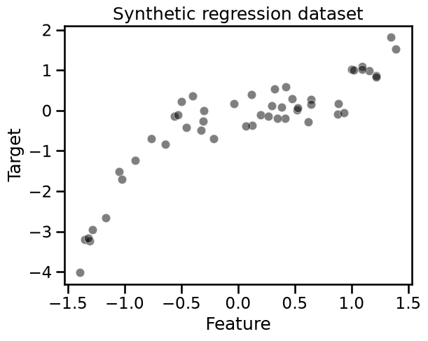
In this section, we provide some intuitions on the way learners are combined to give the final prediction. For such purpose, we tackle a single-feature regression problem, which is more intuitive for demonstrating the underlying machinery.

Later in this notebook we compare the performance of GBDT (boosting) with that of a Random Forest (bagging) for a particular dataset.

import pandas as pd
import numpy as np


def generate_data(n_samples=50):
    """Generate synthetic dataset. Returns `data_train`, `data_test`,
    `target_train`."""
    x_max, x_min = 1.4, -1.4
    rng = np.random.default_rng(0)  # Create a random number generator
    x = rng.uniform(x_min, x_max, size=(n_samples,))
    noise = rng.normal(size=(n_samples,)) * 0.3
    y = x**3 - 0.5 * x**2 + noise

    data_train = pd.DataFrame(x, columns=["Feature"])
    data_test = pd.DataFrame(
        np.linspace(x_max, x_min, num=300), columns=["Feature"]
    )
    target_train = pd.Series(y, name="Target")

    return data_train, data_test, target_train


data_train, data_test, target_train = generate_data()

import matplotlib.pyplot as plt
import seaborn as sns

sns.scatterplot(
    x=data_train["Feature"], y=target_train, color="black", alpha=0.5
)
_ = plt.title("Synthetic regression dataset")

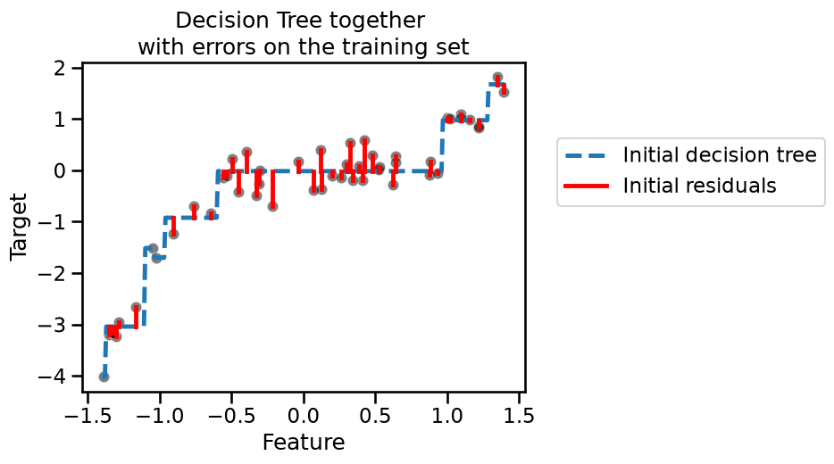
As we previously discussed, boosting is based on assembling a sequence of learners. We start by creating a decision tree regressor. We set the depth of the tree to underfit the data on purpose.

from sklearn.tree import DecisionTreeRegressor

tree = DecisionTreeRegressor(max_depth=3, random_state=0)
tree.fit(data_train, target_train)

target_train_predicted = tree.predict(data_train)
target_test_predicted = tree.predict(data_test)

Using the term “test” here refers to data not used for training. It should not be confused with data coming from a train-test split, as it was generated in equally-spaced intervals for the visual evaluation of the predictions.

To avoid writing the same code in multiple places we define a helper function to plot the data samples as well as the decision tree predictions and residuals.

def plot_decision_tree_with_residuals(y_train, y_train_pred, y_test_pred):
    """Plot the synthetic data, predictions, and residuals for a decision tree.
    Handles are returned to allow custom legends for the plot."""
    _fig_, ax = plt.subplots()
    # plot the data
    sns.scatterplot(
        x=data_train["Feature"], y=y_train, color="black", alpha=0.5, ax=ax
    )
    # plot the predictions
    line_predictions = ax.plot(data_test["Feature"], y_test_pred, "--")

    # plot the residuals
    for value, true, predicted in zip(
        data_train["Feature"], y_train, y_train_pred
    ):
        lines_residuals = ax.plot(
            [value, value], [true, predicted], color="red"
        )

    handles = [line_predictions[0], lines_residuals[0]]

    return handles, ax

handles, ax = plot_decision_tree_with_residuals(
    target_train, target_train_predicted, target_test_predicted
)
legend_labels = ["Initial decision tree", "Initial residuals"]
ax.legend(handles, legend_labels, bbox_to_anchor=(1.05, 0.8), loc="upper left")
_ = ax.set_title("Decision Tree together \nwith errors on the training set")

Tip

In the cell above, we manually edited the legend to get only a single label for all the residual lines.

Since the tree underfits the data, its accuracy is far from perfect on the training data. We can observe this in the figure above by looking at the difference between the predictions and the ground-truth data. We represent these errors, called “residuals”, using solid red lines.

Indeed, our initial tree is not expressive enough to handle the complexity of the data, as shown by the residuals. In a gradient-boosting algorithm, the idea is to create a second tree which, given the same data, tries to predict the residuals instead of the vector target, i.e. we have a second tree that is able to predict the errors made by the initial tree.

Let’s train such a tree.

residuals = target_train - target_train_predicted

tree_residuals = DecisionTreeRegressor(max_depth=5, random_state=0)
tree_residuals.fit(data_train, residuals)

target_train_predicted_residuals = tree_residuals.predict(data_train)
target_test_predicted_residuals = tree_residuals.predict(data_test)

handles, ax = plot_decision_tree_with_residuals(
    residuals,
    target_train_predicted_residuals,
    target_test_predicted_residuals,
)
legend_labels = [
    "Predicted residuals",
    "Residuals of the\npredicted residuals",
]
ax.legend(handles, legend_labels, bbox_to_anchor=(1.05, 0.8), loc="upper left")
_ = ax.set_title("Prediction of the initial residuals")

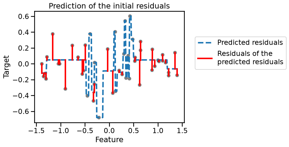
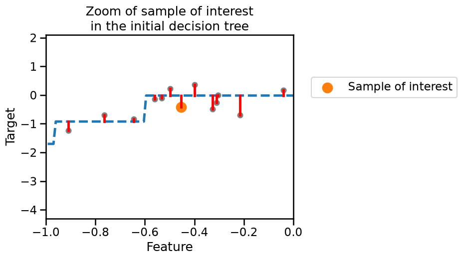
We see that this new tree only manages to fit some of the residuals. We now focus on a specific sample from the training set (as we know that the sample can be well predicted using two successive trees). We will use this sample to explain how the predictions of both trees are combined. Let’s first select this sample in data_train.

sample = data_train.iloc[[-7]]
x_sample = sample["Feature"].iloc[0]
target_true = target_train.iloc[-7]
target_true_residual = residuals.iloc[-7]

Let’s plot the original data, the predictions of the initial decision tree and highlight our sample of interest, i.e. this is just a zoom of the plot displaying the initial shallow tree.

handles, ax = plot_decision_tree_with_residuals(
    target_train, target_train_predicted, target_test_predicted
)
ax.scatter(
    sample, target_true, label="Sample of interest", color="tab:orange", s=200
)
ax.set_xlim([-1, 0])
ax.legend(bbox_to_anchor=(1.05, 0.8), loc="upper left")
_ = ax.set_title("Zoom of sample of interest\nin the initial decision tree")

Similarly we plot a zoom of the plot with the prediction of the initial residuals

handles, ax = plot_decision_tree_with_residuals(
    residuals,
    target_train_predicted_residuals,
    target_test_predicted_residuals,
)
plt.scatter(
    sample,
    target_true_residual,
    label="Sample of interest",
    color="tab:orange",
    s=200,
)
legend_labels = [
    "Predicted residuals",
    "Residuals of the\npredicted residuals",
]
ax.set_xlim([-1, 0])
ax.legend(bbox_to_anchor=(1.05, 0.8), loc="upper left")
_ = ax.set_title("Zoom of sample of interest\nin the initial residuals")

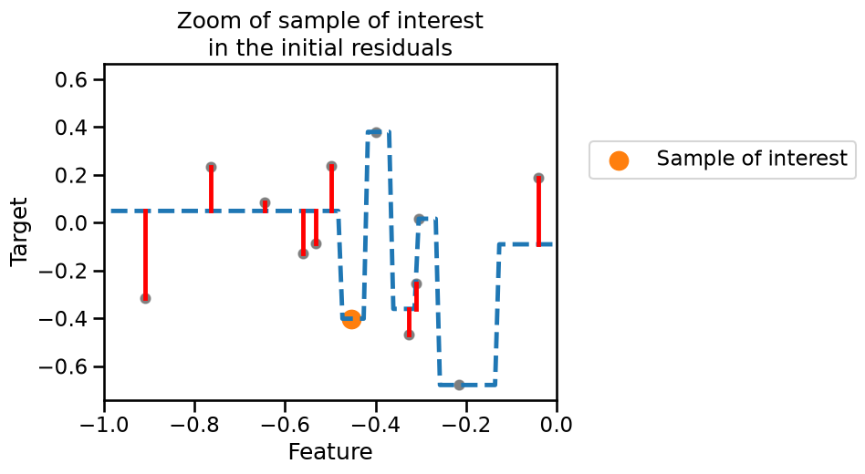
For our sample of interest, our initial tree is making an error (small residual). When fitting the second tree, the residual in this case is perfectly fitted and predicted. We can quantitatively check this prediction using the fitted tree. First, let’s check the prediction of the initial tree and compare it with the true value.

print(f"True value to predict for f(x={x_sample:.3f}) = {target_true:.3f}")

y_pred_first_tree = tree.predict(sample)[0]
print(
    f"Prediction of the first decision tree for x={x_sample:.3f}: "
    f"y={y_pred_first_tree:.3f}"
)
print(f"Error of the tree: {target_true - y_pred_first_tree:.3f}")

True value to predict for f(x=-0.454) = -0.417
Prediction of the first decision tree for x=-0.454: y=-0.016
Error of the tree: -0.401

As we visually observed, we have a small error. Now, we can use the second tree to try to predict this residual.

print(
    f"Prediction of the residual for x={x_sample:.3f}: "
    f"{tree_residuals.predict(sample)[0]:.3f}"
)

Prediction of the residual for x=-0.454: -0.401

We see that our second tree is capable of predicting the exact residual (error) of our first tree. Therefore, we can predict the value of x by summing the prediction of all the trees in the ensemble.

y_pred_first_and_second_tree = (
    y_pred_first_tree + tree_residuals.predict(sample)[0]
)
print(
    "Prediction of the first and second decision trees combined for "
    f"x={x_sample:.3f}: y={y_pred_first_and_second_tree:.3f}"
)
print(f"Error of the tree: {target_true - y_pred_first_and_second_tree:.3f}")

Prediction of the first and second decision trees combined for x=-0.454: y=-0.417
Error of the tree: 0.000

We chose a sample for which only two trees were enough to make the perfect prediction. However, we saw in the previous plot that two trees were not enough to correct the residuals of all samples. Therefore, one needs to add several trees to the ensemble to successfully correct the error (i.e. the second tree corrects the first tree’s error, while the third tree corrects the second tree’s error and so on).

First comparison of GBDT vs. random forests

We now compare the generalization performance of random-forest and gradient boosting on the California housing dataset.

from sklearn.datasets import fetch_california_housing
from sklearn.model_selection import cross_validate

data, target = fetch_california_housing(return_X_y=True, as_frame=True)
target *= 100  # rescale the target in k$

from sklearn.ensemble import GradientBoostingRegressor

gradient_boosting = GradientBoostingRegressor(n_estimators=200)
cv_results_gbdt = cross_validate(
    gradient_boosting,
    data,
    target,
    scoring="neg_mean_absolute_error",
    n_jobs=2,
)

print("Gradient Boosting Decision Tree")
print(
    "Mean absolute error via cross-validation: "
    f"{-cv_results_gbdt['test_score'].mean():.3f} ± "
    f"{cv_results_gbdt['test_score'].std():.3f} k$"
)
print(f"Average fit time: {cv_results_gbdt['fit_time'].mean():.3f} seconds")
print(
    f"Average score time: {cv_results_gbdt['score_time'].mean():.3f} seconds"
)

Gradient Boosting Decision Tree
Mean absolute error via cross-validation: 46.408 ± 2.912 k$
Average fit time: 7.110 seconds
Average score time: 0.008 seconds

from sklearn.ensemble import RandomForestRegressor

random_forest = RandomForestRegressor(n_estimators=200, n_jobs=2)
cv_results_rf = cross_validate(
    random_forest,
    data,
    target,
    scoring="neg_mean_absolute_error",
    n_jobs=2,
)

print("Random Forest")
print(
    "Mean absolute error via cross-validation: "
    f"{-cv_results_rf['test_score'].mean():.3f} ± "
    f"{cv_results_rf['test_score'].std():.3f} k$"
)
print(f"Average fit time: {cv_results_rf['fit_time'].mean():.3f} seconds")
print(f"Average score time: {cv_results_rf['score_time'].mean():.3f} seconds")

Random Forest
Mean absolute error via cross-validation: 46.615 ± 4.742 k$
Average fit time: 12.323 seconds
Average score time: 0.088 seconds

In terms of computing performance, the forest can be parallelized and then benefit from using multiple cores of the CPU. In terms of scoring performance, both algorithms lead to very close results.

However, we see that gradient boosting is overall faster than random forest. One of the reasons is that random forests typically rely on deep trees (that overfit individually) whereas boosting models build shallow trees (that underfit individually) which are faster to fit and predict. In the following exercise we will explore more in depth how these two models compare.