Adaptive Boosting (AdaBoost)

In this notebook, we present the Adaptive Boosting (AdaBoost) algorithm. The aim is to get intuitions regarding the internal machinery of AdaBoost and boosting in general.

We will load the “penguin” dataset. We will predict penguin species from the culmen length and depth features.

import pandas as pd

penguins = pd.read_csv("../datasets/penguins_classification.csv")
culmen_columns = ["Culmen Length (mm)", "Culmen Depth (mm)"]
target_column = "Species"

data, target = penguins[culmen_columns], penguins[target_column]

Note

If you want a deeper overview regarding this dataset, you can refer to the Appendix - Datasets description section at the end of this MOOC.

We will purposefully train a shallow decision tree. Since it is shallow, it is unlikely to overfit and some of the training examples will even be misclassified.

import seaborn as sns
from sklearn.tree import DecisionTreeClassifier

palette = ["tab:red", "tab:blue", "black"]

tree = DecisionTreeClassifier(max_depth=2, random_state=0)
tree.fit(data, target)

DecisionTreeClassifier(max_depth=2, random_state=0)

In a Jupyter environment, please rerun this cell to show the HTML representation or trust the notebook.
On GitHub, the HTML representation is unable to render, please try loading this page with nbviewer.org.

We can predict on the same dataset and check which samples are misclassified.

import numpy as np

target_predicted = tree.predict(data)
misclassified_samples_idx = np.flatnonzero(target != target_predicted)
data_misclassified = data.iloc[misclassified_samples_idx]

import matplotlib.pyplot as plt
from sklearn.inspection import DecisionBoundaryDisplay

DecisionBoundaryDisplay.from_estimator(
    tree, data, response_method="predict", cmap="RdBu", alpha=0.5
)

# plot the original dataset
sns.scatterplot(
    data=penguins,
    x=culmen_columns[0],
    y=culmen_columns[1],
    hue=target_column,
    palette=palette,
)
# plot the misclassified samples
sns.scatterplot(
    data=data_misclassified,
    x=culmen_columns[0],
    y=culmen_columns[1],
    label="Misclassified samples",
    marker="+",
    s=150,
    color="k",
)

plt.legend(bbox_to_anchor=(1.04, 0.5), loc="center left")
_ = plt.title(
    "Decision tree predictions \nwith misclassified samples highlighted"
)

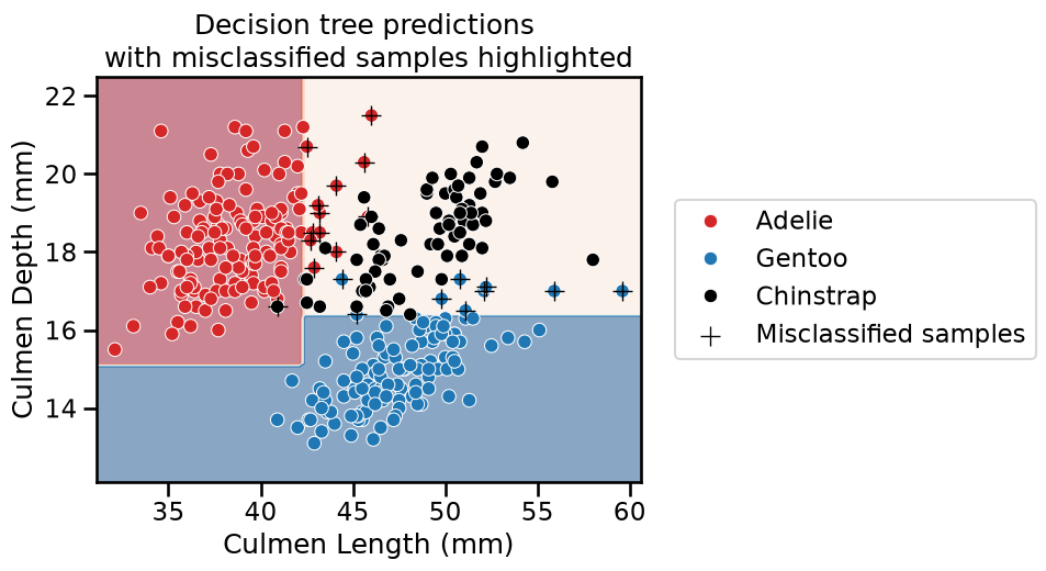
We observe that several samples have been misclassified by the classifier.

We mentioned that boosting relies on creating a new classifier which tries to correct these misclassifications. In scikit-learn, learners have a parameter sample_weight which forces it to pay more attention to samples with higher weights during the training.

This parameter is set when calling classifier.fit(X, y, sample_weight=weights). We will use this trick to create a new classifier by ‘discarding’ all correctly classified samples and only considering the misclassified samples. Thus, misclassified samples will be assigned a weight of 1 and well classified samples will be assigned a weight of 0.

sample_weight = np.zeros_like(target, dtype=int)
sample_weight[misclassified_samples_idx] = 1

tree = DecisionTreeClassifier(max_depth=2, random_state=0)
tree.fit(data, target, sample_weight=sample_weight)

DecisionTreeClassifier(max_depth=2, random_state=0)

In a Jupyter environment, please rerun this cell to show the HTML representation or trust the notebook.
On GitHub, the HTML representation is unable to render, please try loading this page with nbviewer.org.

DecisionBoundaryDisplay.from_estimator(
    tree, data, response_method="predict", cmap="RdBu", alpha=0.5
)
sns.scatterplot(
    data=penguins,
    x=culmen_columns[0],
    y=culmen_columns[1],
    hue=target_column,
    palette=palette,
)
sns.scatterplot(
    data=data_misclassified,
    x=culmen_columns[0],
    y=culmen_columns[1],
    label="Previously misclassified samples",
    marker="+",
    s=150,
    color="k",
)

plt.legend(bbox_to_anchor=(1.04, 0.5), loc="center left")
_ = plt.title("Decision tree by changing sample weights")

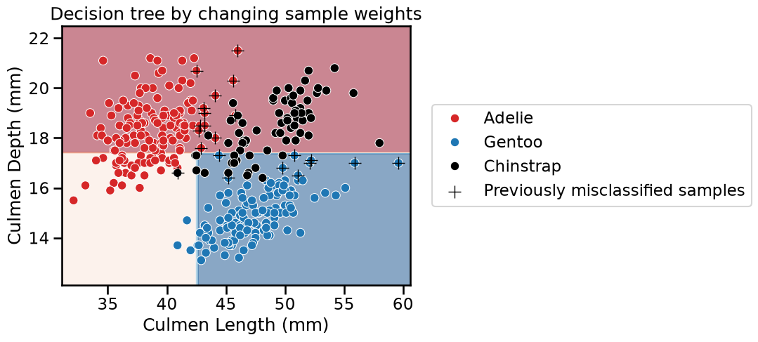
We see that the decision function drastically changed. Qualitatively, we see that the previously misclassified samples are now correctly classified.

target_predicted = tree.predict(data)
newly_misclassified_samples_idx = np.flatnonzero(target != target_predicted)
remaining_misclassified_samples_idx = np.intersect1d(
    misclassified_samples_idx, newly_misclassified_samples_idx
)

print(
    "Number of samples previously misclassified and "
    f"still misclassified: {len(remaining_misclassified_samples_idx)}"
)

Number of samples previously misclassified and still misclassified: 0

However, we are making mistakes on previously well classified samples. Thus, we get the intuition that we should weight the predictions of each classifier differently, most probably by using the number of mistakes each classifier is making.

So we could use the classification error to combine both trees.

ensemble_weight = [
    (target.shape[0] - len(misclassified_samples_idx)) / target.shape[0],
    (target.shape[0] - len(newly_misclassified_samples_idx)) / target.shape[0],
]
ensemble_weight

[0.935672514619883, 0.6929824561403509]

The first classifier was 94% accurate and the second one 69% accurate. Therefore, when predicting a class, we should trust the first classifier slightly more than the second one. We could use these accuracy values to weight the predictions of each learner.

To summarize, boosting learns several classifiers, each of which will focus more or less on specific samples of the dataset. Boosting is thus different from bagging: here we never resample our dataset, we just assign different weights to the original dataset.

Boosting requires some strategy to combine the learners together:

• one needs to define a way to compute the weights to be assigned to samples;

• one needs to assign a weight to each learner when making predictions.

Indeed, we defined a really simple scheme to assign sample weights and learner weights. However, there are statistical theories (like in AdaBoost) for how these sample and learner weights can be optimally calculated.

We will use the AdaBoost classifier implemented in scikit-learn and look at the underlying decision tree classifiers trained.

from sklearn.ensemble import AdaBoostClassifier

estimator = DecisionTreeClassifier(max_depth=3, random_state=0)
adaboost = AdaBoostClassifier(
    estimator=estimator, n_estimators=3, algorithm="SAMME", random_state=0
)
adaboost.fit(data, target)

AdaBoostClassifier(algorithm='SAMME',
                   estimator=DecisionTreeClassifier(max_depth=3,
                                                    random_state=0),
                   n_estimators=3, random_state=0)

In a Jupyter environment, please rerun this cell to show the HTML representation or trust the notebook.
On GitHub, the HTML representation is unable to render, please try loading this page with nbviewer.org.

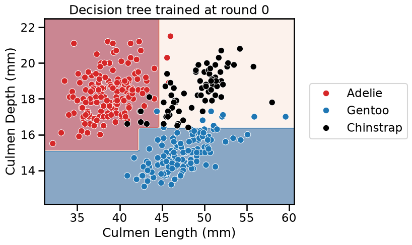
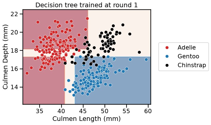
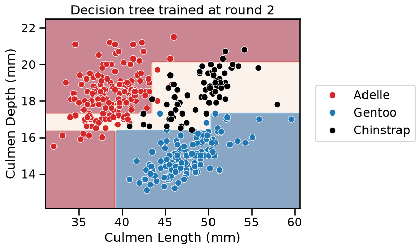
for boosting_round, tree in enumerate(adaboost.estimators_):
    plt.figure()
    # we convert `data` into a NumPy array to avoid a warning raised in scikit-learn
    DecisionBoundaryDisplay.from_estimator(
        tree,
        data.to_numpy(),
        response_method="predict",
        cmap="RdBu",
        alpha=0.5,
    )
    sns.scatterplot(
        x=culmen_columns[0],
        y=culmen_columns[1],
        hue=target_column,
        data=penguins,
        palette=palette,
    )
    plt.legend(bbox_to_anchor=(1.04, 0.5), loc="center left")
    _ = plt.title(f"Decision tree trained at round {boosting_round}")

<Figure size 640x480 with 0 Axes>

<Figure size 640x480 with 0 Axes>

<Figure size 640x480 with 0 Axes>

print(f"Weight of each classifier: {adaboost.estimator_weights_}")

Weight of each classifier: [3.58351894 3.46901998 3.03303773]

print(f"Error of each classifier: {adaboost.estimator_errors_}")

Error of each classifier: [0.05263158 0.05864198 0.08787269]

We see that AdaBoost learned three different classifiers, each of which focuses on different samples. Looking at the weights of each learner, we see that the ensemble gives the highest weight to the first classifier. This indeed makes sense when we look at the errors of each classifier. The first classifier also has the highest classification generalization performance.

While AdaBoost is a nice algorithm to demonstrate the internal machinery of boosting algorithms, it is not the most efficient. This title is handed to the gradient-boosting decision tree (GBDT) algorithm, which we will discuss in the next unit.