📃 Solution for Exercise M2.01

The aim of this exercise is to make the following experiments:

• train and test a support vector machine classifier through cross-validation;

• study the effect of the parameter gamma of this classifier using a validation curve;

• use a learning curve to determine the usefulness of adding new samples in the dataset when building a classifier.

To make these experiments we will first load the blood transfusion dataset.

Note

If you want a deeper overview regarding this dataset, you can refer to the Appendix - Datasets description section at the end of this MOOC.

import pandas as pd

blood_transfusion = pd.read_csv("../datasets/blood_transfusion.csv")
data = blood_transfusion.drop(columns="Class")
target = blood_transfusion["Class"]

We will use a support vector machine classifier (SVM). In its most simple form, a SVM classifier is a linear classifier behaving similarly to a logistic regression. Indeed, the optimization used to find the optimal weights of the linear model are different but we don’t need to know these details for the exercise.

Also, this classifier can become more flexible/expressive by using a so-called kernel that makes the model become non-linear. Again, no requirement regarding the mathematics is required to accomplish this exercise.

We will use an RBF kernel where a parameter gamma allows to tune the flexibility of the model.

First let’s create a predictive pipeline made of:

• a sklearn.preprocessing.StandardScaler with default parameter;

• a sklearn.svm.SVC where the parameter kernel could be set to "rbf". Note that this is the default.

# solution
from sklearn.pipeline import make_pipeline
from sklearn.preprocessing import StandardScaler
from sklearn.svm import SVC

model = make_pipeline(StandardScaler(), SVC())

Evaluate the generalization performance of your model by cross-validation with a ShuffleSplit scheme. Thus, you can use sklearn.model_selection.cross_validate and pass a sklearn.model_selection.ShuffleSplit to the cv parameter. Only fix the random_state=0 in the ShuffleSplit and let the other parameters to the default.

# solution
from sklearn.model_selection import cross_validate, ShuffleSplit

cv = ShuffleSplit(random_state=0)
cv_results = cross_validate(model, data, target, cv=cv, n_jobs=2)
cv_results = pd.DataFrame(cv_results)
cv_results

	fit_time	score_time	test_score
0	0.016879	0.002918	0.680000
1	0.016258	0.002914	0.746667
2	0.015917	0.002771	0.786667
3	0.014870	0.002757	0.800000
4	0.015813	0.002932	0.746667
5	0.015684	0.002934	0.786667
6	0.015162	0.002912	0.800000
7	0.014370	0.002792	0.826667
8	0.015085	0.002710	0.746667
9	0.015120	0.002753	0.733333

print(
    f"Accuracy score of our model:\n"
    f"{cv_results['test_score'].mean():.3f} ± "
    f"{cv_results['test_score'].std():.3f}"
)

Accuracy score of our model:
0.765 ± 0.043

As previously mentioned, the parameter gamma is one of the parameters controlling under/over-fitting in support vector machine with an RBF kernel.

Evaluate the effect of the parameter gamma by using the sklearn.model_selection.validation_curve function. You can leave the default scoring=None which is equivalent to scoring="accuracy" for classification problems. You can vary gamma between 10e-3 and 10e2 by generating samples on a logarithmic scale with the help of np.logspace(-3, 2, num=30).

Since we are manipulating a Pipeline the parameter name will be set to svc__gamma instead of only gamma. You can retrieve the parameter name using model.get_params().keys(). We will go more into detail regarding accessing and setting hyperparameter in the next section.

# solution
import numpy as np
from sklearn.model_selection import validation_curve

gammas = np.logspace(-3, 2, num=30)
param_name = "svc__gamma"
train_scores, test_scores = validation_curve(
    model, data, target, param_name=param_name, param_range=gammas, cv=cv,
    n_jobs=2)

Plot the validation curve for the train and test scores.

# solution
import matplotlib.pyplot as plt

plt.errorbar(
    gammas,
    train_scores.mean(axis=1),
    yerr=train_scores.std(axis=1),
    alpha=0.95,
    label="Training score",
)
plt.errorbar(
    gammas,
    test_scores.mean(axis=1),
    yerr=test_scores.std(axis=1),
    alpha=0.5,
    label="Testing score",
)
plt.legend()

plt.xscale("log")
plt.xlabel(r"Value of hyperparameter $\gamma$")
plt.ylabel("Accuracy score")
_ = plt.title("Validation score of support vector machine")

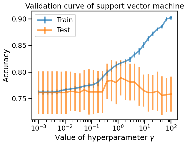
Looking at the curve, we can clearly identify the over-fitting regime of the SVC classifier when gamma > 1. The best setting is around gamma = 1 while for gamma < 1, it is not very clear if the classifier is under-fitting but the testing score is worse than for gamma = 1.

Now, you can perform an analysis to check whether adding new samples to the dataset could help our model to better generalize. Compute the learning curve (using sklearn.model_selection.learning_curve) by computing the train and test scores for different training dataset size. Plot the train and test scores with respect to the number of samples.

# solution
from sklearn.model_selection import learning_curve

train_sizes = np.linspace(0.1, 1, num=10)
results = learning_curve(
    model, data, target, train_sizes=train_sizes, cv=cv, n_jobs=2)
train_size, train_scores, test_scores = results[:3]

plt.errorbar(
    train_size,
    train_scores.mean(axis=1),
    yerr=train_scores.std(axis=1),
    alpha=0.95,
    label="Training score",
)
plt.errorbar(
    train_size,
    test_scores.mean(axis=1),
    yerr=test_scores.std(axis=1),
    alpha=0.5,
    label="Testing score",
)
plt.legend(bbox_to_anchor=(1.05, 0.8), loc="upper left")

plt.xlabel("Number of samples in the training set")
plt.ylabel("Accuracy")
_ = plt.title("Learning curve for support vector machine")

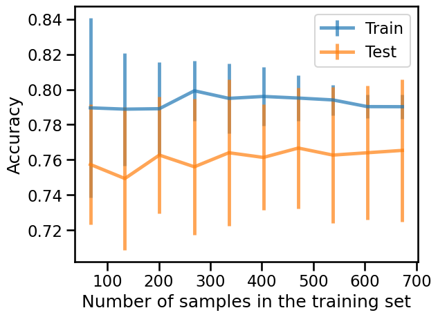
We observe that adding new samples to the training dataset does not seem to improve the training and testing scores. In particular, the testing score oscillates around 76% accuracy. Indeed, ~76% of the samples belong to the class "not donated". Notice then that a classifier that always predicts the "not donated" class would achieve an accuracy of 76% without using any information from the data itself. This can mean that our small pipeline is not able to use the input features to improve upon that simplistic baseline, and increasing the training set size does not help either.

It could be the case that the input features are fundamentally not very informative and the classification problem is fundamentally impossible to solve to a high accuracy. But it could also be the case that our choice of using the default hyperparameter value of the SVC class was a bad idea, or that the choice of the SVC class is itself sub-optimal.

Later in this MOOC we will see how to better tune the hyperparameters of a model and explore how to compare the predictive performance of different model classes in a more systematic way.