The California housing dataset

In this notebook, we will quickly present the dataset known as the “California housing dataset”. This dataset can be fetched from internet using scikit-learn.

from sklearn.datasets import fetch_california_housing

california_housing = fetch_california_housing(as_frame=True)

We can have a first look at the available description

print(california_housing.DESCR)

.. _california_housing_dataset:

California Housing dataset
--------------------------

**Data Set Characteristics:**

:Number of Instances: 20640

:Number of Attributes: 8 numeric, predictive attributes and the target

:Attribute Information:
    - MedInc        median income in block group
    - HouseAge      median house age in block group
    - AveRooms      average number of rooms per household
    - AveBedrms     average number of bedrooms per household
    - Population    block group population
    - AveOccup      average number of household members
    - Latitude      block group latitude
    - Longitude     block group longitude

:Missing Attribute Values: None

This dataset was obtained from the StatLib repository.
https://www.dcc.fc.up.pt/~ltorgo/Regression/cal_housing.html

The target variable is the median house value for California districts,
expressed in hundreds of thousands of dollars ($100,000).

This dataset was derived from the 1990 U.S. census, using one row per census
block group. A block group is the smallest geographical unit for which the U.S.
Census Bureau publishes sample data (a block group typically has a population
of 600 to 3,000 people).

A household is a group of people residing within a home. Since the average
number of rooms and bedrooms in this dataset are provided per household, these
columns may take surprisingly large values for block groups with few households
and many empty houses, such as vacation resorts.

It can be downloaded/loaded using the
:func:`sklearn.datasets.fetch_california_housing` function.

.. rubric:: References

- Pace, R. Kelley and Ronald Barry, Sparse Spatial Autoregressions,
  Statistics and Probability Letters, 33 (1997) 291-297

Let’s have an overview of the entire dataset.

california_housing.frame.head()

	MedInc	HouseAge	AveRooms	AveBedrms	Population	AveOccup	Latitude	Longitude	MedHouseVal
0	8.3252	41.0	6.984127	1.023810	322.0	2.555556	37.88	-122.23	4.526
1	8.3014	21.0	6.238137	0.971880	2401.0	2.109842	37.86	-122.22	3.585
2	7.2574	52.0	8.288136	1.073446	496.0	2.802260	37.85	-122.24	3.521
3	5.6431	52.0	5.817352	1.073059	558.0	2.547945	37.85	-122.25	3.413
4	3.8462	52.0	6.281853	1.081081	565.0	2.181467	37.85	-122.25	3.422

As written in the description, the dataset contains aggregated data regarding each district in California. Let’s have a close look at the features that can be used by a predictive model.

california_housing.data.head()

	MedInc	HouseAge	AveRooms	AveBedrms	Population	AveOccup	Latitude	Longitude
0	8.3252	41.0	6.984127	1.023810	322.0	2.555556	37.88	-122.23
1	8.3014	21.0	6.238137	0.971880	2401.0	2.109842	37.86	-122.22
2	7.2574	52.0	8.288136	1.073446	496.0	2.802260	37.85	-122.24
3	5.6431	52.0	5.817352	1.073059	558.0	2.547945	37.85	-122.25
4	3.8462	52.0	6.281853	1.081081	565.0	2.181467	37.85	-122.25

In this dataset, we have information regarding the demography (income, population, house occupancy) in the districts, the location of the districts (latitude, longitude), and general information regarding the house in the districts (number of rooms, number of bedrooms, age of the house). Since these statistics are at the granularity of the district, they corresponds to averages or medians.

Now, let’s have a look to the target to be predicted.

california_housing.target.head()

0    4.526
1    3.585
2    3.521
3    3.413
4    3.422
Name: MedHouseVal, dtype: float64

The target contains the median of the house value for each district. Therefore, this problem is a regression problem.

We can now check more into details the data types and if the dataset contains any missing value.

california_housing.frame.info()

<class 'pandas.core.frame.DataFrame'>
RangeIndex: 20640 entries, 0 to 20639
Data columns (total 9 columns):
 #   Column       Non-Null Count  Dtype  
---  ------       --------------  -----  
 0   MedInc       20640 non-null  float64
 1   HouseAge     20640 non-null  float64
 2   AveRooms     20640 non-null  float64
 3   AveBedrms    20640 non-null  float64
 4   Population   20640 non-null  float64
 5   AveOccup     20640 non-null  float64
 6   Latitude     20640 non-null  float64
 7   Longitude    20640 non-null  float64
 8   MedHouseVal  20640 non-null  float64
dtypes: float64(9)
memory usage: 1.4 MB

We can see that:

• the dataset contains 20,640 samples and 8 features;

• all features are numerical features encoded as floating number;

• there is no missing values.

Let’s have a quick look at the distribution of these features by plotting their histograms.

import matplotlib.pyplot as plt

california_housing.frame.hist(figsize=(12, 10), bins=30, edgecolor="black")
plt.subplots_adjust(hspace=0.7, wspace=0.4)

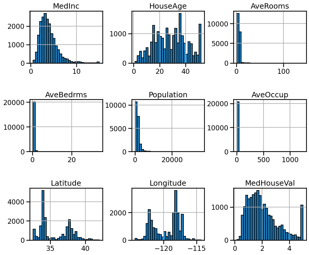
We can first focus on features for which their distributions would be more or less expected.

The median income is a distribution with a long tail. It means that the salary of people is more or less normally distributed but there is some people getting a high salary.

Regarding the average house age, the distribution is more or less uniform.

The target distribution has a long tail as well. In addition, we have a threshold-effect for high-valued houses: all houses with a price above 5 are given the value 5.

Focusing on the average rooms, average bedrooms, average occupation, and population, the range of the data is large with unnoticeable bin for the largest values. It means that there are very high and few values (maybe they could be considered as outliers?). We can see this specificity looking at the statistics for these features:

features_of_interest = ["AveRooms", "AveBedrms", "AveOccup", "Population"]
california_housing.frame[features_of_interest].describe()

	AveRooms	AveBedrms	AveOccup	Population
count	20640.000000	20640.000000	20640.000000	20640.000000
mean	5.429000	1.096675	3.070655	1425.476744
std	2.474173	0.473911	10.386050	1132.462122
min	0.846154	0.333333	0.692308	3.000000
25%	4.440716	1.006079	2.429741	787.000000
50%	5.229129	1.048780	2.818116	1166.000000
75%	6.052381	1.099526	3.282261	1725.000000
max	141.909091	34.066667	1243.333333	35682.000000

For each of these features, comparing the max and 75% values, we can see a huge difference. It confirms the intuitions that there are a couple of extreme values.

Up to know, we discarded the longitude and latitude that carry geographical information. In short, the combination of this feature could help us to decide if there are locations associated with high-valued houses. Indeed, we could make a scatter plot where the x- and y-axis would be the latitude and longitude and the circle size and color would be linked with the house value in the district.

import seaborn as sns

sns.scatterplot(
    data=california_housing.frame,
    x="Longitude",
    y="Latitude",
    size="MedHouseVal",
    hue="MedHouseVal",
    palette="viridis",
    alpha=0.5,
)
plt.legend(title="MedHouseVal", bbox_to_anchor=(1.05, 0.95), loc="upper left")
_ = plt.title("Median house value depending of\n their spatial location")

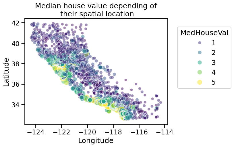
If you are not familiar with the state of California, it is interesting to notice that all datapoints show a graphical representation of this state. We note that the high-valued houses will be located on the coast, where the big cities from California are located: San Diego, Los Angeles, San Jose, or San Francisco.

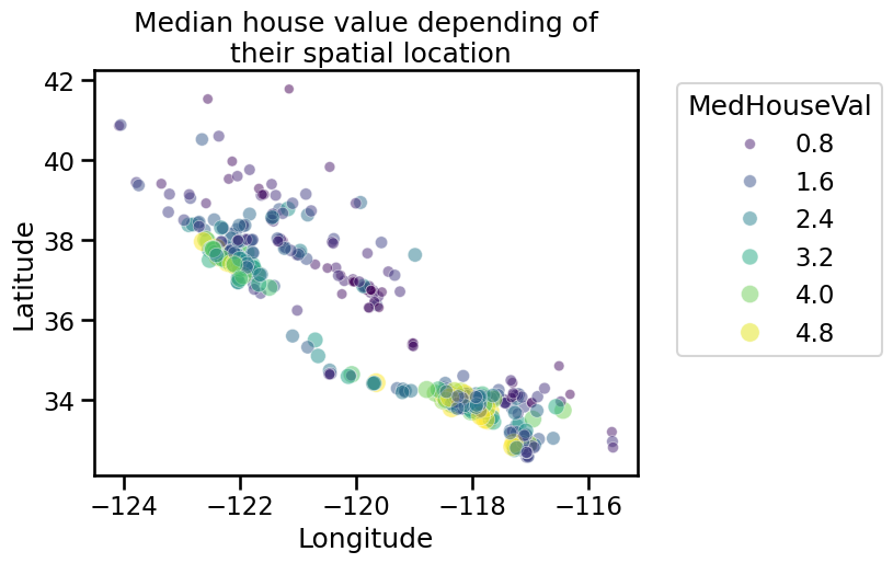
We can do a random subsampling to have less data points to plot but that could still allow us to see these specificities.

import numpy as np

rng = np.random.RandomState(0)
indices = rng.choice(
    np.arange(california_housing.frame.shape[0]), size=500, replace=False
)

sns.scatterplot(
    data=california_housing.frame.iloc[indices],
    x="Longitude",
    y="Latitude",
    size="MedHouseVal",
    hue="MedHouseVal",
    palette="viridis",
    alpha=0.5,
)
plt.legend(title="MedHouseVal", bbox_to_anchor=(1.05, 1), loc="upper left")
_ = plt.title("Median house value depending of\n their spatial location")

We can make a final analysis by making a pair plot of all features and the target but dropping the longitude and latitude. We will quantize the target such that we can create proper histogram.

import pandas as pd

# Drop the unwanted columns
columns_drop = ["Longitude", "Latitude"]
subset = california_housing.frame.iloc[indices].drop(columns=columns_drop)
# Quantize the target and keep the midpoint for each interval
subset["MedHouseVal"] = pd.qcut(subset["MedHouseVal"], 6, retbins=False)
subset["MedHouseVal"] = subset["MedHouseVal"].apply(lambda x: x.mid)

_ = sns.pairplot(data=subset, hue="MedHouseVal", palette="viridis")

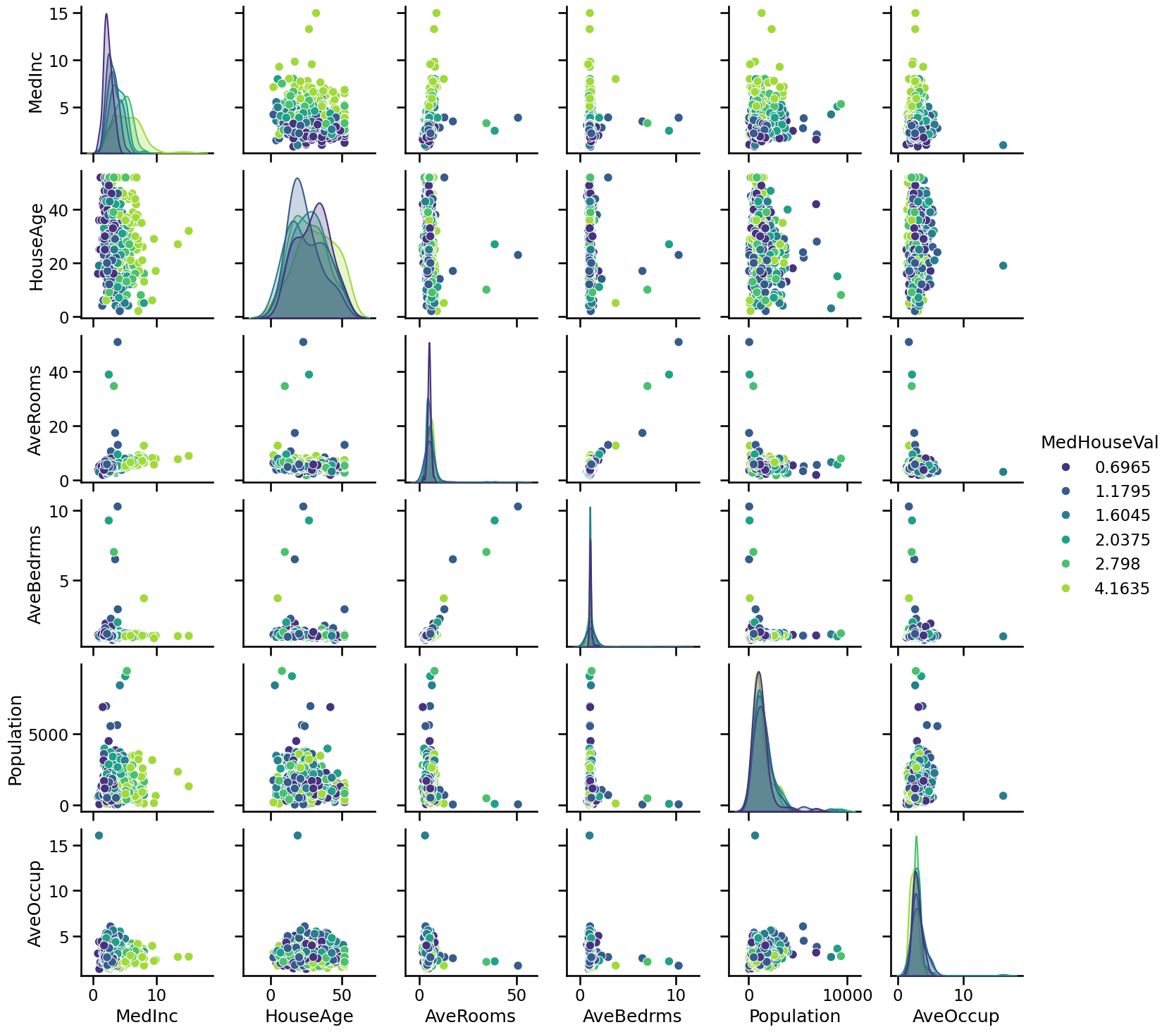
While it is always complicated to interpret a pairplot since there is a lot of data, here we can get a couple of intuitions. We can confirm that some features have extreme values (outliers?). We can as well see that the median income is helpful to distinguish high-valued from low-valued houses.

Thus, creating a predictive model, we could expect the longitude, latitude, and the median income to be useful features to help at predicting the median house values.

If you are curious, we created a linear predictive model below and show the values of the coefficients obtained via cross-validation.

from sklearn.preprocessing import StandardScaler
from sklearn.linear_model import RidgeCV
from sklearn.pipeline import make_pipeline
from sklearn.model_selection import cross_validate

alphas = np.logspace(-3, 1, num=30)
model = make_pipeline(StandardScaler(), RidgeCV(alphas=alphas))
cv_results = cross_validate(
    model,
    california_housing.data,
    california_housing.target,
    return_estimator=True,
    n_jobs=2,
)

score = cv_results["test_score"]
print(f"R2 score: {score.mean():.3f} ± {score.std():.3f}")

R2 score: 0.553 ± 0.062

import pandas as pd

coefs = pd.DataFrame(
    [est[-1].coef_ for est in cv_results["estimator"]],
    columns=california_housing.feature_names,
)

color = {"whiskers": "black", "medians": "black", "caps": "black"}
coefs.plot.box(vert=False, color=color)
plt.axvline(x=0, ymin=-1, ymax=1, color="black", linestyle="--")
_ = plt.title("Coefficients of Ridge models\n via cross-validation")

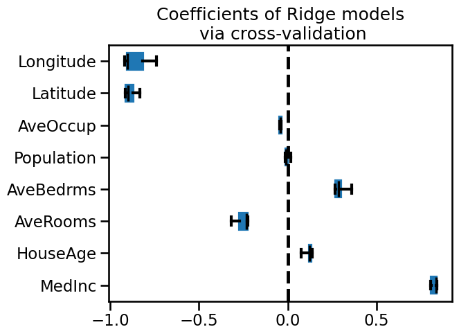
It seems that the three features that we earlier spotted are found important by this model. But be careful regarding interpreting these coefficients. We let you go into the module “Interpretation” to go in depth regarding such experiment.