The bike rides dataset#
In this notebook, we will present the “Bike Ride” dataset. This dataset is
located in the directory datasets in a comma separated values (CSV) format.
We open this dataset using pandas.
import pandas as pd

cycling = pd.read_csv("../datasets/bike_rides.csv")
cycling.head()
| timestamp | power | heart-rate | cadence | speed | acceleration | slope | |
|---|---|---|---|---|---|---|---|
| 0 | 2020-08-18 14:43:19 | 150.0 | 102.0 | 64.0 | 4.325 | 0.0880 | -0.033870 |
| 1 | 2020-08-18 14:43:20 | 161.0 | 103.0 | 64.0 | 4.336 | 0.0842 | -0.033571 |
| 2 | 2020-08-18 14:43:21 | 163.0 | 105.0 | 66.0 | 4.409 | 0.0234 | -0.033223 |
| 3 | 2020-08-18 14:43:22 | 156.0 | 106.0 | 66.0 | 4.445 | 0.0016 | -0.032908 |
| 4 | 2020-08-18 14:43:23 | 148.0 | 106.0 | 67.0 | 4.441 | 0.1144 | 0.000000 |
The first column timestamp contains a specific information regarding the the
time and date of a record while other columns contain numerical value of some
specific measurements. Let’s check the data type of the columns more in
details.
cycling.info()
<class 'pandas.core.frame.DataFrame'>
RangeIndex: 38254 entries, 0 to 38253
Data columns (total 7 columns):
 #   Column        Non-Null Count  Dtype
---  ------        --------------  -----
 0   timestamp     38254 non-null  object
 1   power         38254 non-null  float64
 2   heart-rate    38254 non-null  float64
 3   cadence       38254 non-null  float64
 4   speed         38254 non-null  float64
 5   acceleration  38254 non-null  float64
 6   slope         38254 non-null  float64
dtypes: float64(6), object(1)
memory usage: 2.0+ MB
Indeed, CSV format store data as text. Pandas tries to infer numerical type by
default. It is the reason why all features but timestamp are encoded as
floating point values. However, we see that the timestamp is stored as an
object column. It means that the data in this column are stored as str
rather than a specialized datetime data type.
In fact, one needs to set an option such that pandas is directed to infer such
data type when opening the file. In addition, we will want to use timestamp
as an index. Thus, we can reopen the file with some extra arguments to help
pandas at reading properly our CSV file.
cycling = pd.read_csv(
    "../datasets/bike_rides.csv", index_col=0, parse_dates=True
)
cycling.index.name = ""
cycling.head()
| power | heart-rate | cadence | speed | acceleration | slope | |
|---|---|---|---|---|---|---|
| 2020-08-18 14:43:19 | 150.0 | 102.0 | 64.0 | 4.325 | 0.0880 | -0.033870 |
| 2020-08-18 14:43:20 | 161.0 | 103.0 | 64.0 | 4.336 | 0.0842 | -0.033571 |
| 2020-08-18 14:43:21 | 163.0 | 105.0 | 66.0 | 4.409 | 0.0234 | -0.033223 |
| 2020-08-18 14:43:22 | 156.0 | 106.0 | 66.0 | 4.445 | 0.0016 | -0.032908 |
| 2020-08-18 14:43:23 | 148.0 | 106.0 | 67.0 | 4.441 | 0.1144 | 0.000000 |
cycling.info()
<class 'pandas.core.frame.DataFrame'>
DatetimeIndex: 38254 entries, 2020-08-18 14:43:19 to 2020-09-13 14:56:01
Data columns (total 6 columns):
 #   Column        Non-Null Count  Dtype
---  ------        --------------  -----
 0   power         38254 non-null  float64
 1   heart-rate    38254 non-null  float64
 2   cadence       38254 non-null  float64
 3   speed         38254 non-null  float64
 4   acceleration  38254 non-null  float64
 5   slope         38254 non-null  float64
dtypes: float64(6)
memory usage: 2.0 MB
By specifying to pandas to parse the date, we obtain a DatetimeIndex that is
really handy when filtering data based on date.
We can now have a look at the data stored in our dataframe. It will help us to frame the data science problem that we try to solve.
The records correspond at information derived from GPS recordings of a cyclist
(speed, acceleration, slope) and some extra information acquired from
other sensors: heart-rate that corresponds to the number of beats per minute
of the cyclist heart, cadence that is the rate at which a cyclist is turning
the pedals, and power that corresponds to the work required by the cyclist
to go forward.
The power might be slightly an abstract quantity so let’s give a more intuitive explanation.
Let’s take the example of a soup blender that one uses to blend vegetable. The engine of this blender develop an instantaneous power of ~300 Watts to blend the vegetable. Here, our cyclist is just the engine of the blender (at the difference that an average cyclist will develop an instantaneous power around ~150 Watts) and blending the vegetable corresponds to move the cyclist’s bike forward.
Professional cyclists are using power to calibrate their training and track the energy spent during a ride. For instance, riding at a higher power requires more energy and thus, you need to provide resources to create this energy. With human, this resource is food. For our soup blender, this resource can be uranium, petrol, natural gas, coal, etc. Our body serves as a power plant to transform the resources into energy.
The issue with measuring power is linked to the cost of the sensor: a cycling power meter. The cost of such sensor vary from \(400 to \)1000. Thus, our data science problem is quite easy: can we predict instantaneous cyclist power from other (cheaper) sensors.
target_name = "power"
data, target = cycling.drop(columns=target_name), cycling[target_name]
We can have a first look at the target distribution.
import matplotlib.pyplot as plt

target.plot.hist(bins=50, edgecolor="black")
plt.xlabel("Power (W)")
Text(0.5, 0, 'Power (W)')
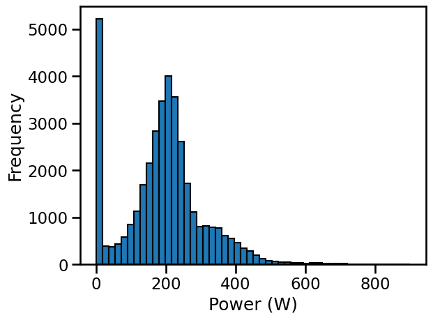
We see a pick at 0 Watts, it corresponds to whenever our cyclist does not pedals (descent, stopped). In average, this cyclist delivers a power around ~200 Watts. We also see a long tail from ~300 Watts to ~400 Watts. You can think that this range of data correspond to effort a cyclist will train to reproduce to be able to breakout in the final kilometers of a cycling race. However, this is costly for the human body and no one can cruise with this power output.
Now, let’s have a look at the data.
data.head()
| heart-rate | cadence | speed | acceleration | slope | |
|---|---|---|---|---|---|
| 2020-08-18 14:43:19 | 102.0 | 64.0 | 4.325 | 0.0880 | -0.033870 |
| 2020-08-18 14:43:20 | 103.0 | 64.0 | 4.336 | 0.0842 | -0.033571 |
| 2020-08-18 14:43:21 | 105.0 | 66.0 | 4.409 | 0.0234 | -0.033223 |
| 2020-08-18 14:43:22 | 106.0 | 66.0 | 4.445 | 0.0016 | -0.032908 |
| 2020-08-18 14:43:23 | 106.0 | 67.0 | 4.441 | 0.1144 | 0.000000 |
We can first have a closer look to the index of the dataframe.
data.index
DatetimeIndex(['2020-08-18 14:43:19', '2020-08-18 14:43:20',
               '2020-08-18 14:43:21', '2020-08-18 14:43:22',
               '2020-08-18 14:43:23', '2020-08-18 14:43:24',
               '2020-08-18 14:43:25', '2020-08-18 14:43:26',
               '2020-08-18 14:43:27', '2020-08-18 14:43:28',
               ...
               '2020-09-13 14:55:52', '2020-09-13 14:55:53',
               '2020-09-13 14:55:54', '2020-09-13 14:55:55',
               '2020-09-13 14:55:56', '2020-09-13 14:55:57',
               '2020-09-13 14:55:58', '2020-09-13 14:55:59',
               '2020-09-13 14:56:00', '2020-09-13 14:56:01'],
              dtype='datetime64[ns]', name='', length=38254, freq=None)
We see that records are acquired every seconds.
data.index.min(), data.index.max()
(Timestamp('2020-08-18 14:43:19'), Timestamp('2020-09-13 14:56:01'))
The starting date is the August 18, 2020 and the ending date is September 13, 2020. However, it is obvious that our cyclist did not ride every seconds between these dates. Indeed, only a couple of date should be present in the dataframe, corresponding to the number of cycling rides.
data.index.normalize().nunique()
4
Indeed, we have only four different dates corresponding to four rides. Let’s extract only the first ride of August 18, 2020.
date_first_ride = "2020-08-18"
cycling_ride = cycling.loc[date_first_ride]
data_ride, target_ride = data.loc[date_first_ride], target.loc[date_first_ride]
data_ride.plot()
plt.legend(bbox_to_anchor=(1.05, 1), loc="upper left")
_ = plt.title("Sensor values for different cyclist measurements")
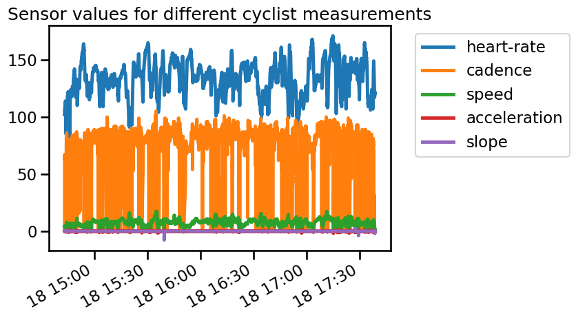
Since the unit and range of each measurement (feature) is different, it is rather difficult to interpret the plot. Also, the high temporal resolution make it difficult to make any observation. We could resample the data to get a smoother visualization.
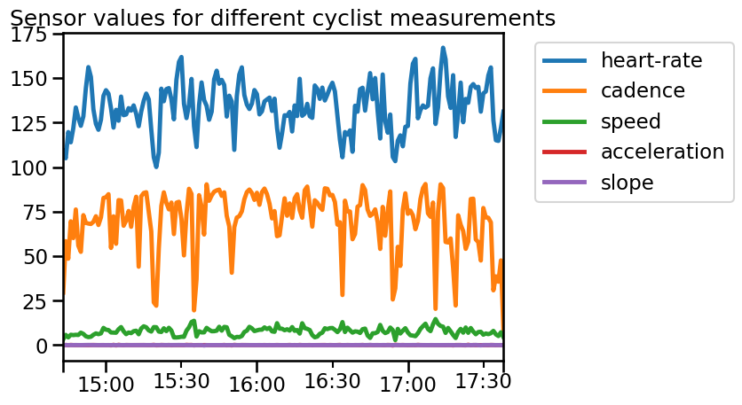
data_ride.resample("60s").mean().plot()
plt.legend(bbox_to_anchor=(1.05, 1), loc="upper left")
_ = plt.title("Sensor values for different cyclist measurements")
We can check the range of the different features:
axs = data_ride.hist(figsize=(10, 12), bins=50, edgecolor="black", grid=False)
# add the units to the plots
units = [
    "beats per minute",
    "rotations per minute",
    "meters per second",
    "meters per second squared",
    "%",
]
for unit, ax in zip(units, axs.ravel()):
    ax.set_xlabel(unit)
plt.subplots_adjust(hspace=0.6)
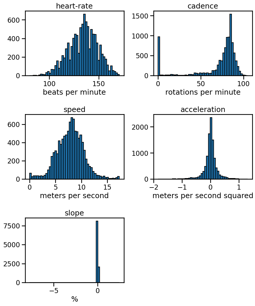
From these plots, we can see some interesting information: a cyclist is spending some time without pedaling. This samples should be associated with a null power. We also see that the slope have large extremum.
Let’s make a pair plot on a subset of data samples to see if we can confirm some of these intuitions.
import numpy as np

rng = np.random.RandomState(0)
indices = rng.choice(np.arange(cycling_ride.shape[0]), size=500, replace=False)
subset = cycling_ride.iloc[indices].copy()
# Quantize the target and keep the midpoint for each interval
subset["power"] = pd.qcut(subset["power"], 6, retbins=False)
subset["power"] = subset["power"].apply(lambda x: x.mid)
import seaborn as sns

_ = sns.pairplot(data=subset, hue="power", palette="viridis")
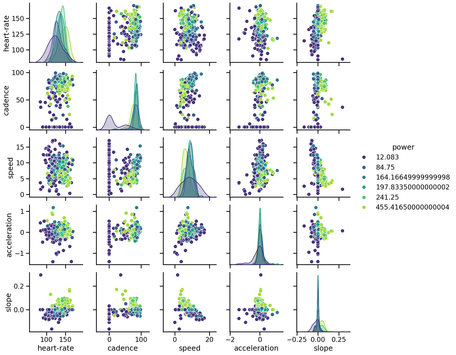
Indeed, we see that low cadence is associated with low power. We can also the a link between higher slope / high heart-rate and higher power: a cyclist need to develop more energy to go uphill enforcing a stronger physiological stimuli on the body. We can confirm this intuition by looking at the interaction between the slope and the speed: a lower speed with a higher slope is usually associated with higher power.