Hyperparameter tuning by grid-search#
In the previous notebook, we saw that hyperparameters can affect the generalization performance of a model. In this notebook, we show how to optimize hyperparameters using a grid-search approach.
Our predictive model#
Let us reload the dataset as we did previously:
import pandas as pd

adult_census = pd.read_csv("../datasets/adult-census.csv")
We extract the column containing the target.
target_name = "class"
target = adult_census[target_name]
target
0         <=50K
1         <=50K
2          >50K
3          >50K
4         <=50K
          ...
48837     <=50K
48838      >50K
48839     <=50K
48840     <=50K
48841      >50K
Name: class, Length: 48842, dtype: object
We drop from our data the target and the "education-num" column which
duplicates the information from the "education" column.
data = adult_census.drop(columns=[target_name, "education-num"])
data
| age | workclass | education | marital-status | occupation | relationship | race | sex | capital-gain | capital-loss | hours-per-week | native-country | |
|---|---|---|---|---|---|---|---|---|---|---|---|---|
| 0 | 25 | Private | 11th | Never-married | Machine-op-inspct | Own-child | Black | Male | 0 | 0 | 40 | United-States |
| 1 | 38 | Private | HS-grad | Married-civ-spouse | Farming-fishing | Husband | White | Male | 0 | 0 | 50 | United-States |
| 2 | 28 | Local-gov | Assoc-acdm | Married-civ-spouse | Protective-serv | Husband | White | Male | 0 | 0 | 40 | United-States |
| 3 | 44 | Private | Some-college | Married-civ-spouse | Machine-op-inspct | Husband | Black | Male | 7688 | 0 | 40 | United-States |
| 4 | 18 | ? | Some-college | Never-married | ? | Own-child | White | Female | 0 | 0 | 30 | United-States |
| ... | ... | ... | ... | ... | ... | ... | ... | ... | ... | ... | ... | ... |
| 48837 | 27 | Private | Assoc-acdm | Married-civ-spouse | Tech-support | Wife | White | Female | 0 | 0 | 38 | United-States |
| 48838 | 40 | Private | HS-grad | Married-civ-spouse | Machine-op-inspct | Husband | White | Male | 0 | 0 | 40 | United-States |
| 48839 | 58 | Private | HS-grad | Widowed | Adm-clerical | Unmarried | White | Female | 0 | 0 | 40 | United-States |
| 48840 | 22 | Private | HS-grad | Never-married | Adm-clerical | Own-child | White | Male | 0 | 0 | 20 | United-States |
| 48841 | 52 | Self-emp-inc | HS-grad | Married-civ-spouse | Exec-managerial | Wife | White | Female | 15024 | 0 | 40 | United-States |
48842 rows × 12 columns
Once the dataset is loaded, we split it into a training and testing sets.
from sklearn.model_selection import train_test_split

data_train, data_test, target_train, target_test = train_test_split(
    data, target, random_state=42
)
We define a pipeline as seen in the first module, to handle both numerical and categorical features.
The first step is to select all the categorical columns.
from sklearn.compose import make_column_selector as selector

categorical_columns_selector = selector(dtype_include=object)
categorical_columns = categorical_columns_selector(data)
Here we use a tree-based model as a classifier (i.e.
HistGradientBoostingClassifier). That means:
Numerical variables don’t need scaling;
Categorical variables can be dealt with an
OrdinalEncodereven if the coding order is not meaningful;For tree-based models, the
OrdinalEncoderavoids having high-dimensional representations.
We now build our OrdinalEncoder by passing it the known categories.
from sklearn.preprocessing import OrdinalEncoder

categorical_preprocessor = OrdinalEncoder(
    handle_unknown="use_encoded_value", unknown_value=-1
)
We then use make_column_transformer to select the categorical columns and apply
the OrdinalEncoder to them.
from sklearn.compose import make_column_transformer

preprocessor = make_column_transformer(
    (categorical_preprocessor, categorical_columns),
    remainder="passthrough",
    # Silence a deprecation warning in scikit-learn v1.6 related to how the
    # ColumnTransformer stores an attribute that we do not use in this notebook
    force_int_remainder_cols=False,
)
Finally, we use a tree-based classifier (i.e. histogram gradient-boosting) to predict whether or not a person earns more than 50 k$ a year.
from sklearn.ensemble import HistGradientBoostingClassifier
from sklearn.pipeline import Pipeline

model = Pipeline(
    [
        ("preprocessor", preprocessor),
        (
            "classifier",
            HistGradientBoostingClassifier(random_state=42, max_leaf_nodes=4),
        ),
    ]
)
model
Pipeline(steps=[('preprocessor',
                 ColumnTransformer(force_int_remainder_cols=False,
                                   remainder='passthrough',
                                   transformers=[('ordinalencoder',
                                                  OrdinalEncoder(handle_unknown='use_encoded_value',
                                                                 unknown_value=-1),
                                                  ['workclass', 'education',
                                                   'marital-status',
                                                   'occupation', 'relationship',
                                                   'race', 'sex',
                                                   'native-country'])])),
                ('classifier',
                 HistGradientBoostingClassifier(max_leaf_nodes=4,
                                                random_state=42))])
In a Jupyter environment, please rerun this cell to show the HTML representation or trust the notebook. On GitHub, the HTML representation is unable to render, please try loading this page with nbviewer.org.
Pipeline(steps=[('preprocessor',
                 ColumnTransformer(force_int_remainder_cols=False,
                                   remainder='passthrough',
                                   transformers=[('ordinalencoder',
                                                  OrdinalEncoder(handle_unknown='use_encoded_value',
                                                                 unknown_value=-1),
                                                  ['workclass', 'education',
                                                   'marital-status',
                                                   'occupation', 'relationship',
                                                   'race', 'sex',
                                                   'native-country'])])),
                ('classifier',
                 HistGradientBoostingClassifier(max_leaf_nodes=4,
random_state=42))])ColumnTransformer(force_int_remainder_cols=False, remainder='passthrough',
transformers=[('ordinalencoder',
OrdinalEncoder(handle_unknown='use_encoded_value',
unknown_value=-1),
['workclass', 'education', 'marital-status',
'occupation', 'relationship', 'race', 'sex',
'native-country'])])['workclass', 'education', 'marital-status', 'occupation', 'relationship', 'race', 'sex', 'native-country']
OrdinalEncoder(handle_unknown='use_encoded_value', unknown_value=-1)
passthrough
HistGradientBoostingClassifier(max_leaf_nodes=4, random_state=42)
Tuning using a grid-search#
In the previous exercise (M3.01) we used two nested for loops (one for each
hyperparameter) to test different combinations over a fixed grid of
hyperparameter values. In each iteration of the loop, we used
cross_val_score to compute the mean score (as averaged across
cross-validation splits), and compared those mean scores to select the best
combination. GridSearchCV is a scikit-learn class that implements a very
similar logic with less repetitive code. The suffix CV refers to the
cross-validation it runs internally (instead of the cross_val_score we
“hard” coded).
The GridSearchCV estimator takes a param_grid parameter which defines all
hyperparameters and their associated values. The grid-search is in charge of
creating all possible combinations and testing them.
The number of combinations is equal to the product of the number of values to explore for each parameter. Thus, adding new parameters with their associated values to be explored rapidly becomes computationally expensive. Because of that, here we only explore the combination learning-rate and the maximum number of nodes for a total of 4 x 3 = 12 combinations.
%%time
from sklearn.model_selection import GridSearchCV
param_grid = {
"classifier__learning_rate": (0.01, 0.1, 1, 10), # 4 possible values
"classifier__max_leaf_nodes": (3, 10, 30), # 3 possible values
} # 12 unique combinations
model_grid_search = GridSearchCV(model, param_grid=param_grid, n_jobs=2, cv=2)
model_grid_search.fit(data_train, target_train)
CPU times: user 1.07 s, sys: 57.6 ms, total: 1.12 s
Wall time: 5.58 s
GridSearchCV(cv=2,
estimator=Pipeline(steps=[('preprocessor',
ColumnTransformer(force_int_remainder_cols=False, remainder='passthrough',
                  transformers=[('ordinalencoder',
                                 OrdinalEncoder(handle_unknown='use_encoded_value',
                                                unknown_value=-1),
                                 ['workclass', 'education', 'marital-status',
                                  'occupation', 'relationship', 'race', 'sex',
'native-country'])])),
('classifier',
HistGradientBoostingClassifier(max_leaf_nodes=4,
random_state=42))]),
n_jobs=2,
param_grid={'classifier__learning_rate': (0.01, 0.1, 1, 10),
'classifier__max_leaf_nodes': (3, 10, 30)})In a Jupyter environment, please rerun this cell to show the HTML representation or trust the notebook. On GitHub, the HTML representation is unable to render, please try loading this page with nbviewer.org.
GridSearchCV(cv=2,
             estimator=Pipeline(steps=[('preprocessor',
                                        ColumnTransformer(force_int_remainder_cols=False,
                                                          remainder='passthrough',
                                                          transformers=[('ordinalencoder',
                                                                         OrdinalEncoder(handle_unknown='use_encoded_value',
                                                                                        unknown_value=-1),
                                                                         ['workclass',
                                                                          'education',
                                                                          'marital-status',
                                                                          'occupation',
                                                                          'relationship',
                                                                          'race',
                                                                          'sex',
                                                                          'native-country'])])),
                                       ('classifier',
                                        HistGradientBoostingClassifier(max_leaf_nodes=4,
                                                                       random_state=42))]),
             n_jobs=2,
             param_grid={'classifier__learning_rate': (0.01, 0.1, 1, 10),
'classifier__max_leaf_nodes': (3, 10, 30)})Pipeline(steps=[('preprocessor',
ColumnTransformer(force_int_remainder_cols=False, remainder='passthrough',
                  transformers=[('ordinalencoder',
                                 OrdinalEncoder(handle_unknown='use_encoded_value',
                                                unknown_value=-1),
                                 ['workclass', 'education', 'marital-status',
                                  'occupation', 'relationship', 'race', 'sex',
'native-country'])])),
('classifier',
HistGradientBoostingClassifier(max_leaf_nodes=30,
random_state=42))])ColumnTransformer(force_int_remainder_cols=False, remainder='passthrough',
transformers=[('ordinalencoder',
OrdinalEncoder(handle_unknown='use_encoded_value',
unknown_value=-1),
['workclass', 'education', 'marital-status',
'occupation', 'relationship', 'race', 'sex',
'native-country'])])['workclass', 'education', 'marital-status', 'occupation', 'relationship', 'race', 'sex', 'native-country']
OrdinalEncoder(handle_unknown='use_encoded_value', unknown_value=-1)
['age', 'capital-gain', 'capital-loss', 'hours-per-week']
passthrough
HistGradientBoostingClassifier(max_leaf_nodes=30, random_state=42)
You can access the best combination of hyperparameters found by the grid
search using the best_params_ attribute.
print(f"The best set of parameters is: {model_grid_search.best_params_}")
The best set of parameters is: {'classifier__learning_rate': 0.1, 'classifier__max_leaf_nodes': 30}
Once the grid-search is fitted, it can be used as any other estimator, i.e. it
has predict and score methods. Internally, it uses the model with the
best parameters found during fit.
Let’s get the predictions for the 5 first samples using the estimator with the best parameters:
model_grid_search.predict(data_test.iloc[0:5])
array([' <=50K', ' <=50K', ' >50K', ' <=50K', ' >50K'], dtype=object)
Finally, we check the accuracy of our model using the test set.
accuracy = model_grid_search.score(data_test, target_test)
print(
    f"The test accuracy score of the grid-search pipeline is: {accuracy:.2f}"
)
The test accuracy score of the grid-search pipeline is: 0.88
The accuracy and the best parameters of the grid-search pipeline are similar
to the ones we found in the previous exercise, where we searched the best
parameters “by hand” through a double for loop.
The need for a validation set#
In the previous section, the selection of the best hyperparameters was done using the train set, coming from the initial train-test split. Then, we evaluated the generalization performance of our tuned model on the left out test set. This can be shown schematically as follows:
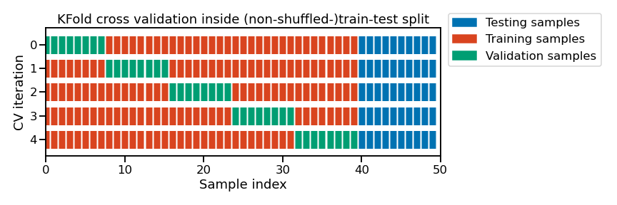
Note
This figure shows the particular case of K-fold cross-validation strategy
using n_splits=5 to further split the train set coming from a train-test
split. For each cross-validation split, the procedure trains a model on all
the red samples, evaluates the score of a given set of hyperparameters on the
green samples. The best combination of hyperparameters best_params is selected
based on those intermediate scores.
Then a final model is refitted using best_params on the concatenation of the
red and green samples and evaluated on the blue samples.
The green samples are sometimes referred as the validation set to differentiate them from the final test set in blue.
In addition, we can inspect all results which are stored in the attribute
cv_results_ of the grid-search. We filter some specific columns from these
results.
cv_results = pd.DataFrame(model_grid_search.cv_results_).sort_values(
    "mean_test_score", ascending=False
)
cv_results
| mean_fit_time | std_fit_time | mean_score_time | std_score_time | param_classifier__learning_rate | param_classifier__max_leaf_nodes | params | split0_test_score | split1_test_score | mean_test_score | std_test_score | rank_test_score | |
|---|---|---|---|---|---|---|---|---|---|---|---|---|
| 5 | 0.363231 | 0.031831 | 0.183779 | 0.008990 | 0.10 | 30 | {'classifier__learning_rate': 0.1, 'classifier... | 0.868912 | 0.867213 | 0.868063 | 0.000850 | 1 |
| 4 | 0.286093 | 0.003133 | 0.163596 | 0.001750 | 0.10 | 10 | {'classifier__learning_rate': 0.1, 'classifier... | 0.866783 | 0.866066 | 0.866425 | 0.000359 | 2 |
| 7 | 0.095261 | 0.003113 | 0.061129 | 0.003788 | 1.00 | 10 | {'classifier__learning_rate': 1, 'classifier__... | 0.854826 | 0.862899 | 0.858863 | 0.004036 | 3 |
| 6 | 0.124936 | 0.028592 | 0.067932 | 0.010819 | 1.00 | 3 | {'classifier__learning_rate': 1, 'classifier__... | 0.853844 | 0.860934 | 0.857389 | 0.003545 | 4 |
| 3 | 0.206374 | 0.000709 | 0.107071 | 0.004051 | 0.10 | 3 | {'classifier__learning_rate': 0.1, 'classifier... | 0.852752 | 0.853781 | 0.853266 | 0.000515 | 5 |
| 8 | 0.105800 | 0.005459 | 0.065354 | 0.002931 | 1.00 | 30 | {'classifier__learning_rate': 1, 'classifier__... | 0.853734 | 0.848321 | 0.851028 | 0.002707 | 6 |
| 2 | 0.458821 | 0.000095 | 0.212328 | 0.007036 | 0.01 | 30 | {'classifier__learning_rate': 0.01, 'classifie... | 0.840413 | 0.846246 | 0.843330 | 0.002917 | 7 |
| 1 | 0.293909 | 0.001703 | 0.166728 | 0.005688 | 0.01 | 10 | {'classifier__learning_rate': 0.01, 'classifie... | 0.818956 | 0.816708 | 0.817832 | 0.001124 | 8 |
| 0 | 0.225017 | 0.000286 | 0.110139 | 0.001610 | 0.01 | 3 | {'classifier__learning_rate': 0.01, 'classifie... | 0.797882 | 0.796451 | 0.797166 | 0.000715 | 9 |
| 10 | 0.067778 | 0.003348 | 0.041420 | 0.000949 | 10.00 | 10 | {'classifier__learning_rate': 10, 'classifier_... | 0.742356 | 0.493803 | 0.618080 | 0.124277 | 10 |
| 11 | 0.065413 | 0.000429 | 0.041804 | 0.001870 | 10.00 | 30 | {'classifier__learning_rate': 10, 'classifier_... | 0.759937 | 0.338739 | 0.549338 | 0.210599 | 11 |
| 9 | 0.064521 | 0.003832 | 0.039807 | 0.001068 | 10.00 | 3 | {'classifier__learning_rate': 10, 'classifier_... | 0.279701 | 0.287251 | 0.283476 | 0.003775 | 12 |
Let us focus on the most interesting columns and shorten the parameter names
to remove the "param_classifier__" prefix for readability:
# get the parameter names
column_results = [f"param_{name}" for name in param_grid.keys()]
column_results += ["mean_test_score", "std_test_score", "rank_test_score"]
cv_results = cv_results[column_results]
def shorten_param(param_name):
    if "__" in param_name:
        return param_name.rsplit("__", 1)[1]
    return param_name


cv_results = cv_results.rename(shorten_param, axis=1)
cv_results
| learning_rate | max_leaf_nodes | mean_test_score | std_test_score | rank_test_score | |
|---|---|---|---|---|---|
| 5 | 0.10 | 30 | 0.868063 | 0.000850 | 1 |
| 4 | 0.10 | 10 | 0.866425 | 0.000359 | 2 |
| 7 | 1.00 | 10 | 0.858863 | 0.004036 | 3 |
| 6 | 1.00 | 3 | 0.857389 | 0.003545 | 4 |
| 3 | 0.10 | 3 | 0.853266 | 0.000515 | 5 |
| 8 | 1.00 | 30 | 0.851028 | 0.002707 | 6 |
| 2 | 0.01 | 30 | 0.843330 | 0.002917 | 7 |
| 1 | 0.01 | 10 | 0.817832 | 0.001124 | 8 |
| 0 | 0.01 | 3 | 0.797166 | 0.000715 | 9 |
| 10 | 10.00 | 10 | 0.618080 | 0.124277 | 10 |
| 11 | 10.00 | 30 | 0.549338 | 0.210599 | 11 |
| 9 | 10.00 | 3 | 0.283476 | 0.003775 | 12 |
Given that we are tuning only 2 parameters, we can visualize the results as a
heatmap. To do so, we first need to reshape the cv_results into a dataframe
where:
the rows correspond to the learning-rate values;
the columns correspond to the maximum number of leaf;
the content of the dataframe is the mean test scores.
pivoted_cv_results = cv_results.pivot_table(
    values="mean_test_score",
    index=["learning_rate"],
    columns=["max_leaf_nodes"],
)

pivoted_cv_results
| max_leaf_nodes | 3 | 10 | 30 |
|---|---|---|---|
| learning_rate | |||
| 0.01 | 0.797166 | 0.817832 | 0.843330 |
| 0.10 | 0.853266 | 0.866425 | 0.868063 |
| 1.00 | 0.857389 | 0.858863 | 0.851028 |
| 10.00 | 0.283476 | 0.618080 | 0.549338 |
Now that we have the data in the right format, we can create the heatmap as follows:
import seaborn as sns

ax = sns.heatmap(
    pivoted_cv_results,
    annot=True,
    cmap="YlGnBu",
    vmin=0.7,
    vmax=0.9,
    cbar_kws={"label": "mean test accuracy"},
)
ax.invert_yaxis()
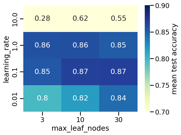
The heatmap above shows the mean test accuracy (i.e., the average over cross-validation splits) for each combination of hyperparameters, where darker colors indicate better performance. However, notice that using colors only allows us to visually compare the mean test score, but does not carry any information on the standard deviation over splits, making it difficult to say if different scores coming from different combinations lead to a significantly better model or not.
The above tables highlights the following things:
for too high values of
learning_rate, the generalization performance of the model is degraded and adjusting the value ofmax_leaf_nodescannot fix that problem;outside of this pathological region, we observe that the optimal choice of
max_leaf_nodesdepends on the value oflearning_rate;in particular, we observe a “diagonal” of good models with an accuracy close to the maximal of 0.87: when the value of
max_leaf_nodesis increased, one should decrease the value oflearning_rateaccordingly to preserve a good accuracy.
The precise meaning of those two parameters will be explained later.
For now we note that, in general, there is no unique optimal parameter setting: 4 models out of the 12 parameter configurations reach the maximal accuracy (up to small random fluctuations caused by the sampling of the training set).
In this notebook we have seen:
how to optimize the hyperparameters of a predictive model via a grid-search;
that searching for more than two hyperparameters is too costly;
that a grid-search does not necessarily find an optimal solution.