Linear regression without scikit-learn

In this notebook, we introduce linear regression. Before presenting the available scikit-learn classes, here we provide some insights with a simple example. We use a dataset that contains measurements taken on penguins.

Note

If you want a deeper overview regarding this dataset, you can refer to the Appendix - Datasets description section at the end of this MOOC.

import pandas as pd

penguins = pd.read_csv("../datasets/penguins_regression.csv")
penguins

	Flipper Length (mm)	Body Mass (g)
0	181.0	3750.0
1	186.0	3800.0
2	195.0	3250.0
3	193.0	3450.0
4	190.0	3650.0
...	...	...
337	207.0	4000.0
338	202.0	3400.0
339	193.0	3775.0
340	210.0	4100.0
341	198.0	3775.0

342 rows × 2 columns

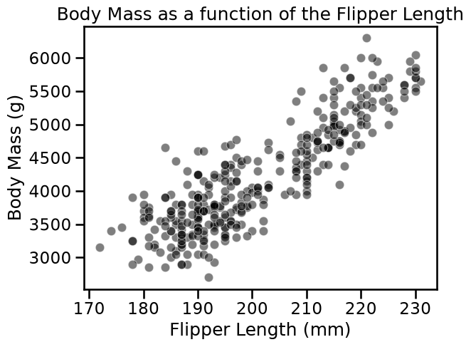
We aim to solve the following problem: using the flipper length of a penguin, we would like to infer its mass.

import seaborn as sns

feature_name = "Flipper Length (mm)"
target_name = "Body Mass (g)"
data, target = penguins[[feature_name]], penguins[target_name]

ax = sns.scatterplot(
    data=penguins, x=feature_name, y=target_name, color="black", alpha=0.5
)
ax.set_title("Body Mass as a function of the Flipper Length")

Text(0.5, 1.0, 'Body Mass as a function of the Flipper Length')

Tip

The function scatterplot from seaborn take as input the full dataframe and the parameter x and y allows to specify the name of the columns to be plotted. Note that this function returns a matplotlib axis (named ax in the example above) that can be further used to add elements on the same matplotlib axis (such as a title).

In this problem, penguin mass is our target. It is a continuous variable that roughly varies between 2700 g and 6300 g. Thus, this is a regression problem (in contrast to classification). We also see that there is almost a linear relationship between the body mass of the penguin and its flipper length. The longer the flipper, the heavier the penguin.

Thus, we could come up with a simple formula, where given a flipper length we could compute the body mass of a penguin using a linear relationship of the form y = a * x + b where a and b are the 2 parameters of our model.

def linear_model_flipper_mass(
    flipper_length, weight_flipper_length, intercept_body_mass
):
    """Linear model of the form y = a * x + b"""
    body_mass = weight_flipper_length * flipper_length + intercept_body_mass
    return body_mass

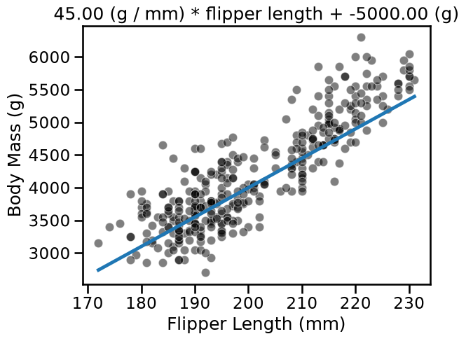
Using the model we defined above, we can check the body mass values predicted for a range of flipper lengths. We set weight_flipper_length and intercept_body_mass to arbitrary values of 45 and -5000, respectively.

import numpy as np

weight_flipper_length = 45
intercept_body_mass = -5000

flipper_length_range = np.linspace(data.min(), data.max(), num=300)
predicted_body_mass = linear_model_flipper_mass(
    flipper_length_range, weight_flipper_length, intercept_body_mass
)

We can now plot all samples and the linear model prediction.

label = "{0:.2f} (g / mm) * flipper length + {1:.2f} (g)"

ax = sns.scatterplot(
    data=penguins, x=feature_name, y=target_name, color="black", alpha=0.5
)
ax.plot(flipper_length_range, predicted_body_mass)
_ = ax.set_title(label.format(weight_flipper_length, intercept_body_mass))

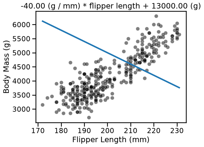
The variable weight_flipper_length is a weight applied to the feature flipper_length in order to make the inference. When this coefficient is positive, it means that penguins with longer flipper lengths have larger body masses. If the coefficient is negative, it means that penguins with shorter flipper lengths have larger body masses. Graphically, this coefficient is represented by the slope of the curve in the plot. Below we show what the curve would look like when the weight_flipper_length coefficient is negative.

weight_flipper_length = -40
intercept_body_mass = 13000

predicted_body_mass = linear_model_flipper_mass(
    flipper_length_range, weight_flipper_length, intercept_body_mass
)

We can now plot all samples and the linear model prediction.

ax = sns.scatterplot(
    data=penguins, x=feature_name, y=target_name, color="black", alpha=0.5
)
ax.plot(flipper_length_range, predicted_body_mass)
_ = ax.set_title(label.format(weight_flipper_length, intercept_body_mass))

In our case, this coefficient has a meaningful unit: g/mm. For instance, a coefficient of 40 g/mm, means that for each additional millimeter in flipper length, the body weight predicted increases by 40 g.

body_mass_180 = linear_model_flipper_mass(
    flipper_length=180, weight_flipper_length=40, intercept_body_mass=0
)
body_mass_181 = linear_model_flipper_mass(
    flipper_length=181, weight_flipper_length=40, intercept_body_mass=0
)

print(
    "The body mass for a flipper length of 180 mm "
    f"is {body_mass_180} g and {body_mass_181} g "
    "for a flipper length of 181 mm"
)

The body mass for a flipper length of 180 mm is 7200 g and 7240 g for a flipper length of 181 mm

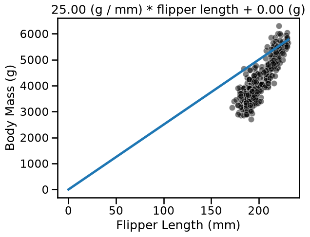
We can also see that we have a parameter intercept_body_mass in our model. This parameter corresponds to the value on the y-axis if flipper_length=0 (which in our case is only a mathematical consideration, as in our data, the value of flipper_length only goes from 170mm to 230mm). This y-value when x=0 is called the y-intercept. If intercept_body_mass is 0, the curve passes through the origin:

weight_flipper_length = 25
intercept_body_mass = 0

# redefined the flipper length to start at 0 to plot the intercept value
flipper_length_range = np.linspace(0, data.max(), num=300)
predicted_body_mass = linear_model_flipper_mass(
    flipper_length_range, weight_flipper_length, intercept_body_mass
)

ax = sns.scatterplot(
    data=penguins, x=feature_name, y=target_name, color="black", alpha=0.5
)
ax.plot(flipper_length_range, predicted_body_mass)
_ = ax.set_title(label.format(weight_flipper_length, intercept_body_mass))

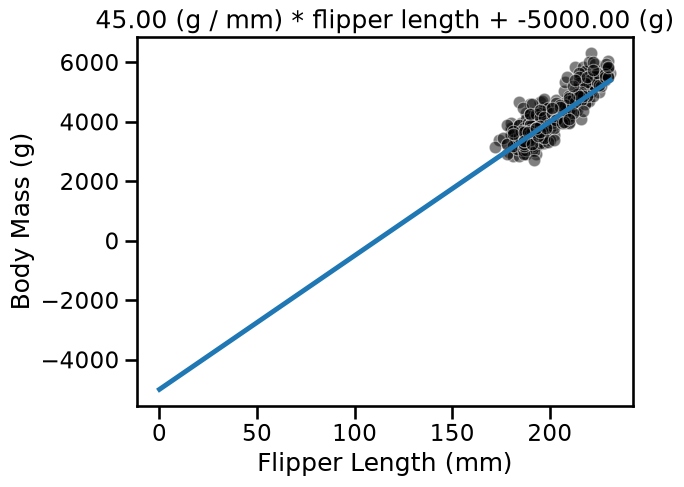
Otherwise, it passes through the intercept_body_mass value:

weight_flipper_length = 45
intercept_body_mass = -5000

predicted_body_mass = linear_model_flipper_mass(
    flipper_length_range, weight_flipper_length, intercept_body_mass
)

ax = sns.scatterplot(
    data=penguins, x=feature_name, y=target_name, color="black", alpha=0.5
)
ax.plot(flipper_length_range, predicted_body_mass)
_ = ax.set_title(label.format(weight_flipper_length, intercept_body_mass))

In this notebook, we have seen the parametrization of a linear regression model and more precisely meaning of the terms weights and intercepts.