The blood transfusion dataset

In this notebook, we will present the “blood transfusion” dataset. This dataset is locally available in the directory datasets and it is stored as a comma separated value (CSV) file. We start by loading the entire dataset.

import pandas as pd

blood_transfusion = pd.read_csv("../datasets/blood_transfusion.csv")

We can have a first look at the at the dataset loaded.

blood_transfusion.head()

	Recency	Frequency	Monetary	Time	Class
0	2	50	12500	98	donated
1	0	13	3250	28	donated
2	1	16	4000	35	donated
3	2	20	5000	45	donated
4	1	24	6000	77	not donated

In this dataframe, we can see that the last column correspond to the target to be predicted called "Class". We will create two variables, data and target to separate the data from which we could learn a predictive model and the target that should be predicted.

data = blood_transfusion.drop(columns="Class")
target = blood_transfusion["Class"]

Let’s have a first look at the data variable.

data.head()

	Recency	Frequency	Monetary	Time
0	2	50	12500	98
1	0	13	3250	28
2	1	16	4000	35
3	2	20	5000	45
4	1	24	6000	77

We observe four columns. Each record corresponds to a person that intended to give blood. The information stored in each column are:

• Recency: the time in months since the last time a person intended to give blood;

• Frequency: the number of time a person intended to give blood in the past;

• Monetary: the amount of blood given in the past (in cm³);

• Time: the time in months since the first time a person intended to give blood.

Now, let’s have a look regarding the type of data that we are dealing in these columns and if any missing values are present in our dataset.

data.info()

<class 'pandas.core.frame.DataFrame'>
RangeIndex: 748 entries, 0 to 747
Data columns (total 4 columns):
 #   Column     Non-Null Count  Dtype
---  ------     --------------  -----
 0   Recency    748 non-null    int64
 1   Frequency  748 non-null    int64
 2   Monetary   748 non-null    int64
 3   Time       748 non-null    int64
dtypes: int64(4)
memory usage: 23.5 KB

Our dataset is made of 748 samples. All features are represented with integer numbers and there is no missing values. We can have a look at each feature distributions.

_ = data.hist(figsize=(12, 10), bins=30, edgecolor="black")

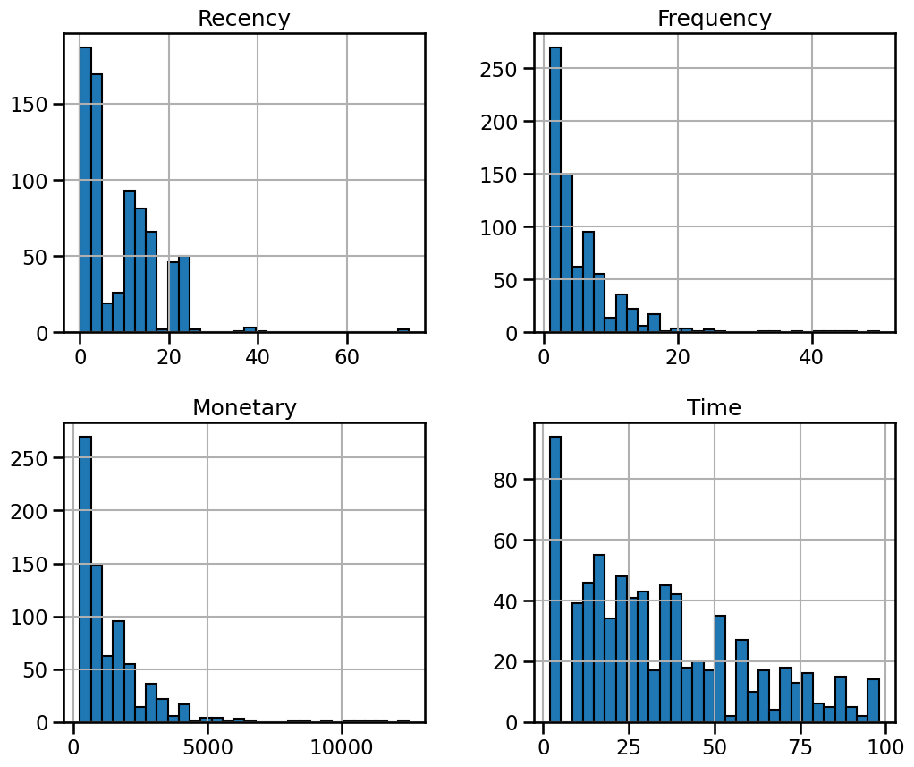
There is nothing shocking regarding the distributions. We only observe a high value range for the features "Recency", "Frequency", and "Monetary". It means that we have a few extreme high values for these features.

Now, let’s have a look at the target that we would like to predict for this task.

target.head()

0        donated
1        donated
2        donated
3        donated
4    not donated
Name: Class, dtype: object

import matplotlib.pyplot as plt

target.value_counts(normalize=True).plot.barh()
plt.xlabel("Number of samples")
_ = plt.title("Class distribution")

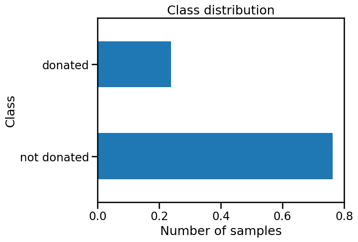
We see that the target is discrete and contains two categories: whether a person "donated" or "not donated" his/her blood. Thus the task to be solved is a classification problem. We should note that the class counts of these two classes is different.

target.value_counts(normalize=True)

Class
not donated    0.762032
donated        0.237968
Name: proportion, dtype: float64

Indeed, ~76% of the samples belong to the class "not donated". It is rather important: a classifier that would predict always this "not donated" class would achieve an accuracy of 76% of good classification without using any information from the data itself. This issue is known as class imbalance. One should take care about the generalization performance metric used to evaluate a model as well as the predictive model chosen itself.

Now, let’s have a naive analysis to see if there is a link between features and the target using a pair plot representation.

import seaborn as sns

_ = sns.pairplot(blood_transfusion, hue="Class")

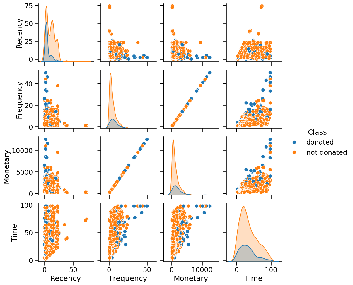
Looking at the diagonal plots, we don’t see any feature that individually could help at separating the two classes. When looking at a pair of feature, we don’t see any striking combinations as well. However, we can note that the "Monetary" and "Frequency" features are perfectly correlated: all the data points are aligned on a diagonal.

As a conclusion, this dataset would be a challenging dataset: it suffer from class imbalance, correlated features and thus very few features will be available to learn a model, and none of the feature combinations were found to help at predicting.