Feature importance

In this notebook, we will detail methods to investigate the importance of features used by a given model. We will look at:

1. interpreting the coefficients in a linear model;

2. the attribute feature_importances_ in RandomForest;

3. permutation feature importance, which is an inspection technique that can be used for any fitted model.

0. Presentation of the dataset

This dataset is a record of neighborhoods in California district, predicting the median house value (target) given some information about the neighborhoods, as the average number of rooms, the latitude, the longitude or the median income of people in the neighborhoods (block).

from sklearn.datasets import fetch_california_housing
import pandas as pd

X, y = fetch_california_housing(as_frame=True, return_X_y=True)

To speed up the computation, we take the first 10000 samples

X = X[:10000]
y = y[:10000]

X.head()

	MedInc	HouseAge	AveRooms	AveBedrms	Population	AveOccup	Latitude	Longitude
0	8.3252	41.0	6.984127	1.023810	322.0	2.555556	37.88	-122.23
1	8.3014	21.0	6.238137	0.971880	2401.0	2.109842	37.86	-122.22
2	7.2574	52.0	8.288136	1.073446	496.0	2.802260	37.85	-122.24
3	5.6431	52.0	5.817352	1.073059	558.0	2.547945	37.85	-122.25
4	3.8462	52.0	6.281853	1.081081	565.0	2.181467	37.85	-122.25

The feature reads as follow:

• MedInc: median income in block

• HouseAge: median house age in block

• AveRooms: average number of rooms

• AveBedrms: average number of bedrooms

• Population: block population

• AveOccup: average house occupancy

• Latitude: house block latitude

• Longitude: house block longitude

• MedHouseVal: Median house value in 100k$ (target)

To assert the quality of our inspection technique, let’s add some random feature that won’t help the prediction (un-informative feature)

import numpy as np

# Adding random features
rng = np.random.RandomState(0)
bin_var = pd.Series(rng.randint(0, 1, X.shape[0]), name="rnd_bin")
num_var = pd.Series(np.arange(X.shape[0]), name="rnd_num")
X_with_rnd_feat = pd.concat((X, bin_var, num_var), axis=1)

We will split the data into training and testing for the remaining part of this notebook

from sklearn.model_selection import train_test_split

X_train, X_test, y_train, y_test = train_test_split(
    X_with_rnd_feat, y, random_state=29
)

Let’s quickly inspect some features and the target:

import seaborn as sns

train_dataset = X_train.copy()
train_dataset.insert(0, "MedHouseVal", y_train)
_ = sns.pairplot(
    train_dataset[
        ["MedHouseVal", "Latitude", "AveRooms", "AveBedrms", "MedInc"]
    ],
    kind="reg",
    diag_kind="kde",
    plot_kws={"scatter_kws": {"alpha": 0.1}},
)

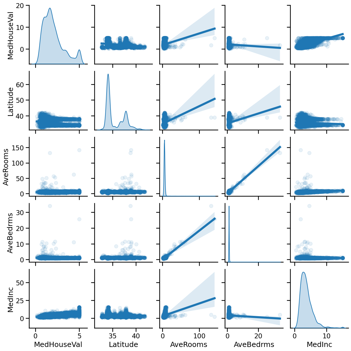
We see in the upper right plot that the median income seems to be positively correlated to the median house price (the target).

We can also see that the average number of rooms AveRooms is very correlated to the average number of bedrooms AveBedrms.

1. Linear model inspection

In linear models, the target value is modeled as a linear combination of the features.

Coefficients represent the relationship between the given feature \(X_i\) and the target \(y\), assuming that all the other features remain constant (conditional dependence). This is different from plotting \(X_i\) versus \(y\) and fitting a linear relationship: in that case all possible values of the other features are taken into account in the estimation (marginal dependence).

from sklearn.linear_model import RidgeCV

model = RidgeCV()

model.fit(X_train, y_train)

print(f"model score on training data: {model.score(X_train, y_train)}")
print(f"model score on testing data: {model.score(X_test, y_test)}")

model score on training data: 0.6013465986314437
model score on testing data: 0.5975758025570992

Our linear model obtains a \(R^2\) score of .60, so it explains a significant part of the target. Its coefficient should be somehow relevant. Let’s look at the coefficient learnt:

import matplotlib.pyplot as plt

coefs = pd.DataFrame(
    model.coef_, columns=["Coefficients"], index=X_train.columns
)

coefs.plot(kind="barh", figsize=(9, 7))
plt.title("Ridge model")
plt.axvline(x=0, color=".5")
plt.subplots_adjust(left=0.3)

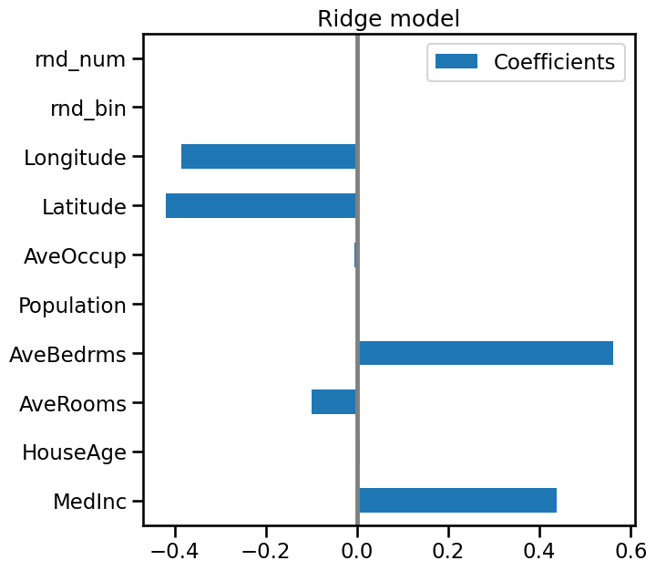
Sign of coefficients

A surprising association?

Why is the coefficient associated to AveRooms negative? Does the price of houses decreases with the number of rooms?

The coefficients of a linear model are a conditional association: they quantify the variation of a the output (the price) when the given feature is varied, keeping all other features constant. We should not interpret them as a marginal association, characterizing the link between the two quantities ignoring all the rest.

The coefficient associated to AveRooms is negative because the number of rooms is strongly correlated with the number of bedrooms, AveBedrms. What we are seeing here is that for districts where the houses have the same number of bedrooms on average, when there are more rooms (hence non-bedroom rooms), the houses are worth comparatively less.

Scale of coefficients

The AveBedrms have the higher coefficient. However, we can’t compare the magnitude of these coefficients directly, since they are not scaled. Indeed, Population is an integer which can be thousands, while AveBedrms is around 4 and Latitude is in degree.

So the Population coefficient is expressed in “\(100k\$\) / habitant” while the AveBedrms is expressed in “\(100k\$\) / nb of bedrooms” and the Latitude coefficient in “\(100k\$\) / degree”.

We see that changing population by one does not change the outcome, while as we go south (latitude increase) the price becomes cheaper. Also, adding a bedroom (keeping all other feature constant) shall rise the price of the house by 80k$.

So looking at the coefficient plot to gauge feature importance can be misleading as some of them vary on a small scale, while others vary a lot more, several decades.

This becomes visible if we compare the standard deviations of our different features.

X_train.std(axis=0).plot(kind="barh", figsize=(9, 7))
plt.title("Features std. dev.")
plt.subplots_adjust(left=0.3)
plt.xlim((0, 100))

(0.0, 100.0)

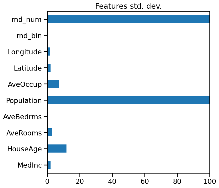
So before any interpretation, we need to scale each column (removing the mean and scaling the variance to 1).

from sklearn.pipeline import make_pipeline
from sklearn.preprocessing import StandardScaler

model = make_pipeline(StandardScaler(), RidgeCV())

model.fit(X_train, y_train)

print(f"model score on training data: {model.score(X_train, y_train)}")
print(f"model score on testing data: {model.score(X_test, y_test)}")

model score on training data: 0.601315755610292
model score on testing data: 0.5972410717953709

coefs = pd.DataFrame(
    model[1].coef_, columns=["Coefficients"], index=X_train.columns
)

coefs.plot(kind="barh", figsize=(9, 7))
plt.title("Ridge model")
plt.axvline(x=0, color=".5")
plt.subplots_adjust(left=0.3)

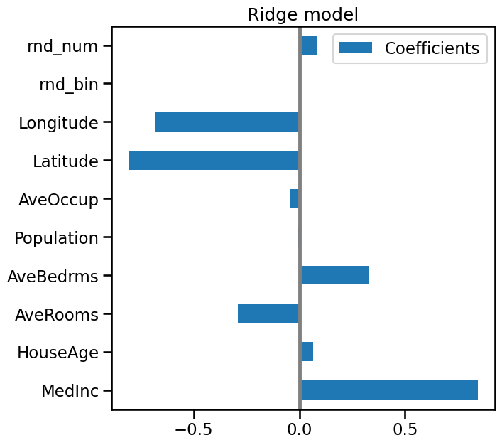
Now that the coefficients have been scaled, we can safely compare them.

The median income feature, with longitude and latitude are the three variables that most influence the model.

The plot above tells us about dependencies between a specific feature and the target when all other features remain constant, i.e., conditional dependencies. An increase of the HouseAge will induce an increase of the price when all other features remain constant. On the contrary, an increase of the average rooms will induce an decrease of the price when all other features remain constant.

Checking the variability of the coefficients

We can check the coefficient variability through cross-validation: it is a form of data perturbation.

If coefficients vary significantly when changing the input dataset their robustness is not guaranteed, and they should probably be interpreted with caution.

from sklearn.model_selection import cross_validate
from sklearn.model_selection import RepeatedKFold

cv_model = cross_validate(
    model,
    X_with_rnd_feat,
    y,
    cv=RepeatedKFold(n_splits=5, n_repeats=5),
    return_estimator=True,
    n_jobs=2,
)
coefs = pd.DataFrame(
    [model[1].coef_ for model in cv_model["estimator"]],
    columns=X_with_rnd_feat.columns,
)
plt.figure(figsize=(9, 7))
sns.boxplot(data=coefs, orient="h", color="cyan", saturation=0.5)
plt.axvline(x=0, color=".5")
plt.xlabel("Coefficient importance")
plt.title("Coefficient importance and its variability")
plt.subplots_adjust(left=0.3)

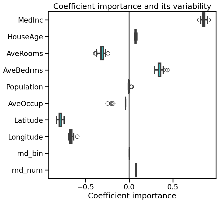
Every coefficient looks pretty stable, which mean that different Ridge model put almost the same weight to the same feature.

Linear models with sparse coefficients (Lasso)

In it important to keep in mind that the associations extracted depend on the model. To illustrate this point we consider a Lasso model, that performs feature selection with a L1 penalty. Let us fit a Lasso model with a strong regularization parameters alpha

from sklearn.linear_model import Lasso

model = make_pipeline(StandardScaler(), Lasso(alpha=0.015))

model.fit(X_train, y_train)

print(f"model score on training data: {model.score(X_train, y_train)}")
print(f"model score on testing data: {model.score(X_test, y_test)}")

model score on training data: 0.5899811014945939
model score on testing data: 0.5769786920519312

coefs = pd.DataFrame(
    model[1].coef_, columns=["Coefficients"], index=X_train.columns
)

coefs.plot(kind="barh", figsize=(9, 7))
plt.title("Lasso model, strong regularization")
plt.axvline(x=0, color=".5")
plt.subplots_adjust(left=0.3)

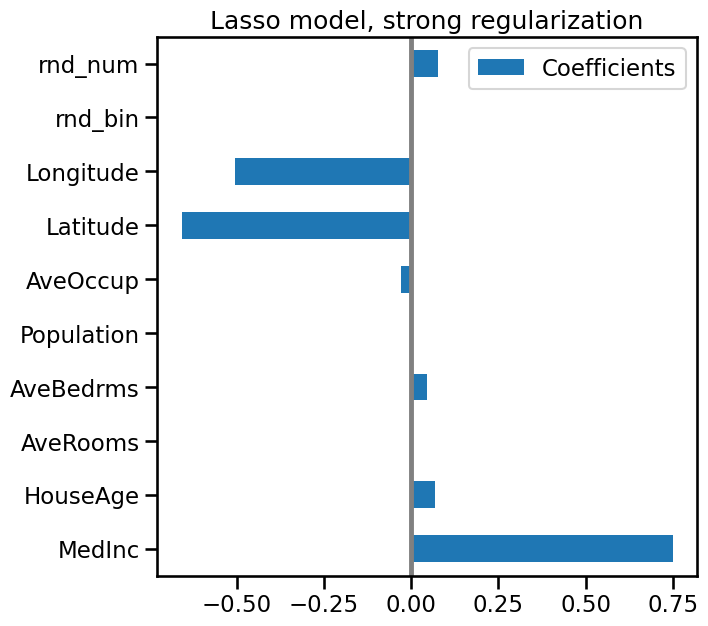
Here the model score is a bit lower, because of the strong regularization. However, it has zeroed out 3 coefficients, selecting a small number of variables to make its prediction.

We can see that out of the two correlated features AveRooms and AveBedrms, the model has selected one. Note that this choice is partly arbitrary: choosing one does not mean that the other is not important for prediction. Avoid over-interpreting models, as they are imperfect.

As above, we can look at the variability of the coefficients:

cv_model = cross_validate(
    model,
    X_with_rnd_feat,
    y,
    cv=RepeatedKFold(n_splits=5, n_repeats=5),
    return_estimator=True,
    n_jobs=2,
)
coefs = pd.DataFrame(
    [model[1].coef_ for model in cv_model["estimator"]],
    columns=X_with_rnd_feat.columns,
)
plt.figure(figsize=(9, 7))
sns.boxplot(data=coefs, orient="h", color="cyan", saturation=0.5)
plt.axvline(x=0, color=".5")
plt.xlabel("Coefficient importance")
plt.title("Coefficient importance and its variability")
plt.subplots_adjust(left=0.3)

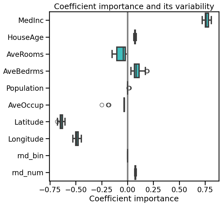
We can see that both the coefficients associated to AveRooms and AveBedrms have a strong variability and that they can both be non zero. Given that they are strongly correlated, the model can pick one or the other to predict well. This choice is a bit arbitrary, and must not be over-interpreted.

Lessons learned

Coefficients must be scaled to the same unit of measure to retrieve feature importance, or comparing them.

Coefficients in multivariate linear models represent the dependency between a given feature and the target, conditional on the other features.

Correlated features might induce instabilities in the coefficients of linear models and their effects cannot be well teased apart.

Inspecting coefficients across the folds of a cross-validation loop gives an idea of their stability.

2. RandomForest feature_importances_

On some algorithms, there are some feature importance methods, inherently built within the model. It is the case in RandomForest models. Let’s investigate the built-in feature_importances_ attribute.

from sklearn.ensemble import RandomForestRegressor

model = RandomForestRegressor()

model.fit(X_train, y_train)

print(f"model score on training data: {model.score(X_train, y_train)}")
print(f"model score on testing data: {model.score(X_test, y_test)}")

model score on training data: 0.979644258021242
model score on testing data: 0.8473167534323301

Contrary to the testing set, the score on the training set is almost perfect, which means that our model is overfitting here.

importances = model.feature_importances_

The importance of a feature is basically: how much this feature is used in each tree of the forest. Formally, it is computed as the (normalized) total reduction of the criterion brought by that feature.

indices = np.argsort(importances)

fig, ax = plt.subplots()
ax.barh(range(len(importances)), importances[indices])
ax.set_yticks(range(len(importances)))
_ = ax.set_yticklabels(np.array(X_train.columns)[indices])

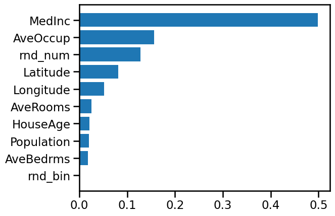
Median income is still the most important feature.

It also has a small bias toward high cardinality features, such as the noisy feature rnd_num, which are here predicted having .07 importance, more than HouseAge (which has low cardinality).

3. Feature importance by permutation

We introduce here a new technique to evaluate the feature importance of any given fitted model. It basically shuffles a feature and sees how the model changes its prediction. Thus, the change in prediction will correspond to the feature importance.

# Any model could be used here

model = RandomForestRegressor()
# model = make_pipeline(StandardScaler(),
#                       RidgeCV())

model.fit(X_train, y_train)

print(f"model score on training data: {model.score(X_train, y_train)}")
print(f"model score on testing data: {model.score(X_test, y_test)}")

model score on training data: 0.9794815819760767
model score on testing data: 0.8480236800534244

As the model gives a good prediction, it has captured well the link between X and y. Hence, it is reasonable to interpret what it has captured from the data.

Feature importance

Lets compute the feature importance for a given feature, say the MedInc feature.

For that, we will shuffle this specific feature, keeping the other feature as is, and run our same model (already fitted) to predict the outcome. The decrease of the score shall indicate how the model had used this feature to predict the target. The permutation feature importance is defined to be the decrease in a model score when a single feature value is randomly shuffled.

For instance, if the feature is crucial for the model, the outcome would also be permuted (just as the feature), thus the score would be close to zero. Afterward, the feature importance is the decrease in score. So in that case, the feature importance would be close to the score.

On the contrary, if the feature is not used by the model, the score shall remain the same, thus the feature importance will be close to 0.

def get_score_after_permutation(model, X, y, curr_feat):
    """return the score of model when curr_feat is permuted"""

    X_permuted = X.copy()
    col_idx = list(X.columns).index(curr_feat)
    # permute one column
    X_permuted.iloc[:, col_idx] = np.random.permutation(
        X_permuted[curr_feat].values
    )

    permuted_score = model.score(X_permuted, y)
    return permuted_score


def get_feature_importance(model, X, y, curr_feat):
    """compare the score when curr_feat is permuted"""

    baseline_score_train = model.score(X, y)
    permuted_score_train = get_score_after_permutation(model, X, y, curr_feat)

    # feature importance is the difference between the two scores
    feature_importance = baseline_score_train - permuted_score_train
    return feature_importance


curr_feat = "MedInc"

feature_importance = get_feature_importance(model, X_train, y_train, curr_feat)
print(
    f'feature importance of "{curr_feat}" on train set is '
    f"{feature_importance:.3}"
)

feature importance of "MedInc" on train set is 0.679

Since there is some randomness, it is advisable to run it multiple times and inspect the mean and the standard deviation of the feature importance.

n_repeats = 10

list_feature_importance = []
for n_round in range(n_repeats):
    list_feature_importance.append(
        get_feature_importance(model, X_train, y_train, curr_feat)
    )

print(
    f'feature importance of "{curr_feat}" on train set is '
    f"{np.mean(list_feature_importance):.3} "
    f"± {np.std(list_feature_importance):.3}"
)

feature importance of "MedInc" on train set is 0.67 ± 0.0108

0.67 over 0.98 is very relevant (note the \(R^2\) score could go below 0). So we can imagine our model relies heavily on this feature to predict the class. We can now compute the feature permutation importance for all the features.

def permutation_importance(model, X, y, n_repeats=10):
    """Calculate importance score for each feature."""

    importances = []
    for curr_feat in X.columns:
        list_feature_importance = []
        for n_round in range(n_repeats):
            list_feature_importance.append(
                get_feature_importance(model, X, y, curr_feat)
            )

        importances.append(list_feature_importance)

    return {
        "importances_mean": np.mean(importances, axis=1),
        "importances_std": np.std(importances, axis=1),
        "importances": importances,
    }


# This function could directly be access from sklearn
# from sklearn.inspection import permutation_importance

def plot_feature_importances(perm_importance_result, feat_name):
    """bar plot the feature importance"""

    fig, ax = plt.subplots()

    indices = perm_importance_result["importances_mean"].argsort()
    plt.barh(
        range(len(indices)),
        perm_importance_result["importances_mean"][indices],
        xerr=perm_importance_result["importances_std"][indices],
    )

    ax.set_yticks(range(len(indices)))
    _ = ax.set_yticklabels(feat_name[indices])

Let’s compute the feature importance by permutation on the training data.

perm_importance_result_train = permutation_importance(
    model, X_train, y_train, n_repeats=10
)

plot_feature_importances(perm_importance_result_train, X_train.columns)

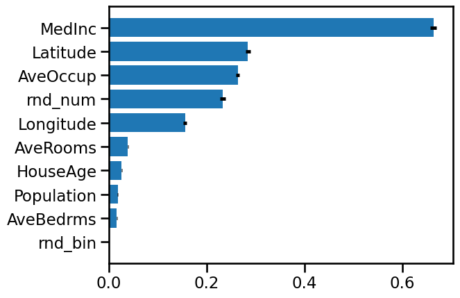
We see again that the feature MedInc, Latitude and Longitude are very important for the model.

We note that our random variable rnd_num is now very less important than latitude. Indeed, the feature importance built-in in RandomForest has bias for continuous data, such as AveOccup and rnd_num.

However, the model still uses these rnd_num feature to compute the output. It is in line with the overfitting we had noticed between the train and test score.

discussion

1. For correlated feature, the permutation could give non realistic sample (e.g. nb of bedrooms higher than the number of rooms)

2. It is unclear whether you should use training or testing data to compute the feature importance.

3. Note that dropping a column and fitting a new model will not allow to analyse the feature importance for a specific model, since a new model will be fitted.

Take Away

• One could directly interpret the coefficient in linear model (if the feature have been scaled first)

• Model like RandomForest have built-in feature importance

• permutation_importance gives feature importance by permutation for any fitted model