Comparing model performance with a simple baseline

In this notebook, we present how to compare the generalization performance of a model to a minimal baseline. In regression, we can use the DummyRegressor class to predict the mean target value observed on the training set without using the input features.

We now demonstrate how to compute the score of a regression model and then compare it to such a baseline on the California housing dataset.

Note

If you want a deeper overview regarding this dataset, you can refer to the section named “Appendix - Datasets description” at the end of this MOOC.

from sklearn.datasets import fetch_california_housing

data, target = fetch_california_housing(return_X_y=True, as_frame=True)
target *= 100  # rescale the target in k$

Across all evaluations, we will use a ShuffleSplit cross-validation splitter with 20% of the data held on the validation side of the split.

from sklearn.model_selection import ShuffleSplit

cv = ShuffleSplit(n_splits=30, test_size=0.2, random_state=0)

We start by running the cross-validation for a simple decision tree regressor which is our model of interest. Besides, we will store the testing error in a pandas series to make it easier to plot the results.

import pandas as pd
from sklearn.tree import DecisionTreeRegressor
from sklearn.model_selection import cross_validate

regressor = DecisionTreeRegressor()
cv_results_tree_regressor = cross_validate(
    regressor, data, target, cv=cv, scoring="neg_mean_absolute_error", n_jobs=2
)

errors_tree_regressor = pd.Series(
    -cv_results_tree_regressor["test_score"], name="Decision tree regressor"
)
errors_tree_regressor.describe()

count    30.000000
mean     45.789573
std       1.230836
min      42.939234
25%      44.946287
50%      45.810916
75%      46.625877
max      48.026353
Name: Decision tree regressor, dtype: float64

Then, we evaluate our baseline. This baseline is called a dummy regressor. This dummy regressor will always predict the mean target computed on the training target variable. Therefore, the dummy regressor does not use any information from the input features stored in the dataframe named data.

from sklearn.dummy import DummyRegressor

dummy = DummyRegressor(strategy="mean")
result_dummy = cross_validate(
    dummy, data, target, cv=cv, scoring="neg_mean_absolute_error", n_jobs=2
)
errors_dummy_regressor = pd.Series(
    -result_dummy["test_score"], name="Dummy regressor"
)
errors_dummy_regressor.describe()

count    30.000000
mean     91.140009
std       0.821140
min      89.757566
25%      90.543652
50%      91.034555
75%      91.979007
max      92.477244
Name: Dummy regressor, dtype: float64

We now plot the cross-validation testing errors for the mean target baseline and the actual decision tree regressor.

all_errors = pd.concat(
    [errors_tree_regressor, errors_dummy_regressor],
    axis=1,
)
all_errors

	Decision tree regressor	Dummy regressor
0	46.674628	90.713153
1	46.787644	90.539353
2	44.500138	91.941912
3	43.408689	90.213912
4	48.026353	92.015862
5	45.504401	90.542490
6	44.208422	89.757566
7	44.883667	92.477244
8	45.134149	90.947952
9	45.241490	91.991373
10	46.479623	92.023571
11	46.309001	90.556965
12	45.690299	91.539567
13	45.679379	91.185225
14	47.520800	92.298971
15	44.331630	91.084639
16	46.235730	90.984471
17	46.983591	89.981744
18	44.820654	90.547140
19	47.076617	89.820219
20	42.939234	91.768721
21	45.704958	92.305556
22	45.896213	90.503017
23	46.750189	92.147974
24	46.361768	91.386320
25	45.919011	90.815660
26	44.668147	92.216574
27	46.274482	90.107460
28	45.725620	90.620318
29	47.950674	91.165331

import matplotlib.pyplot as plt
import numpy as np

bins = np.linspace(start=0, stop=100, num=80)
all_errors.plot.hist(bins=bins, edgecolor="black")
plt.legend(bbox_to_anchor=(1.05, 0.8), loc="upper left")
plt.xlabel("Mean absolute error (k$)")
_ = plt.title("Cross-validation testing errors")

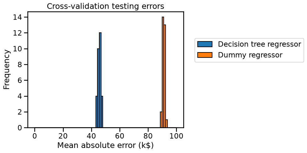
We see that the generalization performance of our decision tree is far from being perfect: the price predictions are off by more than 45,000 US dollars on average. However it is much better than the mean price baseline. So this confirms that it is possible to predict the housing price much better by using a model that takes into account the values of the input features (housing location, size, neighborhood income…). Such a model makes more informed predictions and approximately divides the error rate by a factor of 2 compared to the baseline that ignores the input features.

Note that here we used the mean price as the baseline prediction. We could have used the median instead. See the online documentation of the sklearn.dummy.DummyRegressor class for other options. For this particular example, using the mean instead of the median does not make much of a difference but this could have been the case for dataset with extreme outliers.