Non-linear feature engineering for Logistic Regression

In the slides at the beginning of the module we mentioned that linear classification models are not suited to non-linearly separable data. Nevertheless, one can still use feature engineering as previously done for regression models to overcome this issue. To do so, we use non-linear transformations that typically map the original feature space into a higher dimension space, where the linear model can separate the data more easily.

Let us illustrate this on three synthetic datasets. Each dataset has two original features and two classes to make it easy to visualize. The first dataset is called the “moons” dataset as the data points from each class are shaped as a crescent moon:

import numpy as np
import pandas as pd
from sklearn.datasets import make_moons

feature_names = ["Feature #0", "Feature #1"]
target_name = "class"

X, y = make_moons(n_samples=100, noise=0.13, random_state=42)

# We store both the data and target in a dataframe to ease plotting
moons = pd.DataFrame(
    np.concatenate([X, y[:, np.newaxis]], axis=1),
    columns=feature_names + [target_name],
)
data_moons, target_moons = moons[feature_names], moons[target_name]

The second dataset is called the “Gaussian quantiles” dataset as all data points are sampled from a 2D Gaussian distribution regardless of the class. The points closest to the center are assigned to the class 1 while the points in the outer edges are assigned to the class 0, resulting in concentric circles.

from sklearn.datasets import make_gaussian_quantiles

X, y = make_gaussian_quantiles(
    n_samples=100, n_features=2, n_classes=2, random_state=42
)
gauss = pd.DataFrame(
    np.concatenate([X, y[:, np.newaxis]], axis=1),
    columns=feature_names + [target_name],
)
data_gauss, target_gauss = gauss[feature_names], gauss[target_name]

The third dataset is called the “XOR” dataset as the data points are sampled from a uniform distribution in a 2D space and the class is defined by the Exclusive OR (XOR) operation on the two features: the target class is 1 if only one of the two features is greater than 0. The target class is 0 otherwise.

xor = pd.DataFrame(
    np.random.RandomState(0).uniform(low=-1, high=1, size=(200, 2)),
    columns=feature_names,
)
target_xor = np.logical_xor(xor["Feature #0"] > 0, xor["Feature #1"] > 0)
target_xor = target_xor.astype(np.int32)
xor["class"] = target_xor
data_xor = xor[feature_names]

We use matplotlib to visualize all the datasets at a glance:

import matplotlib.pyplot as plt
from matplotlib.colors import ListedColormap


_, axs = plt.subplots(ncols=3, figsize=(14, 4), constrained_layout=True)

common_scatter_plot_params = dict(
    cmap=ListedColormap(["tab:red", "tab:blue"]),
    edgecolor="white",
    linewidth=1,
)

axs[0].scatter(
    data_moons[feature_names[0]],
    data_moons[feature_names[1]],
    c=target_moons,
    **common_scatter_plot_params,
)
axs[1].scatter(
    data_gauss[feature_names[0]],
    data_gauss[feature_names[1]],
    c=target_gauss,
    **common_scatter_plot_params,
)
axs[2].scatter(
    data_xor[feature_names[0]],
    data_xor[feature_names[1]],
    c=target_xor,
    **common_scatter_plot_params,
)
axs[0].set(
    title="The moons dataset",
    xlabel=feature_names[0],
    ylabel=feature_names[1],
)
axs[1].set(
    title="The Gaussian quantiles dataset",
    xlabel=feature_names[0],
)
axs[2].set(
    title="The XOR dataset",
    xlabel=feature_names[0],
)

[Text(0.5, 1.0, 'The XOR dataset'), Text(0.5, 0, 'Feature #0')]

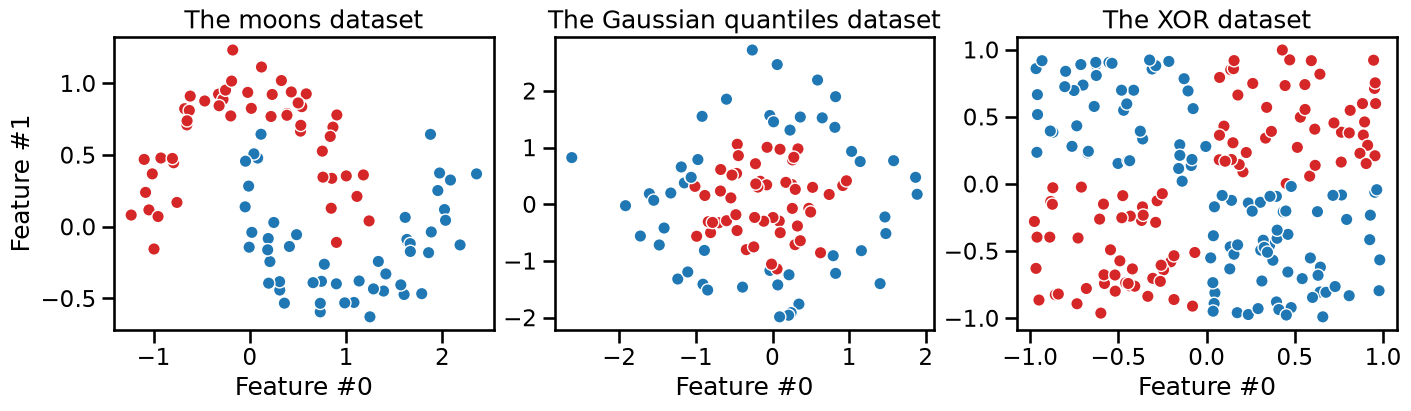
We intuitively observe that there is no (single) straight line that can separate the two classes in any of the datasets. We can confirm this by fitting a linear model, such as a logistic regression, to each dataset and plot the decision boundary of the model.

Let’s first define a function to help us fit a given model and plot its decision boundary on the previous datasets at a glance:

from sklearn.inspection import DecisionBoundaryDisplay


def plot_decision_boundary(model, title=None):
    datasets = [
        (data_moons, target_moons),
        (data_gauss, target_gauss),
        (data_xor, target_xor),
    ]
    fig, axs = plt.subplots(
        ncols=3,
        figsize=(14, 4),
        constrained_layout=True,
    )

    for i, ax, (data, target) in zip(
        range(len(datasets)),
        axs,
        datasets,
    ):
        model.fit(data, target)
        DecisionBoundaryDisplay.from_estimator(
            model,
            data,
            response_method="predict_proba",
            plot_method="pcolormesh",
            cmap="RdBu",
            alpha=0.8,
            # Setting vmin and vmax to the extreme values of the probability to
            # ensure that 0.5 is mapped to white (the middle) of the blue-red
            # colormap.
            vmin=0,
            vmax=1,
            ax=ax,
        )
        DecisionBoundaryDisplay.from_estimator(
            model,
            data,
            response_method="predict_proba",
            plot_method="contour",
            alpha=0.8,
            levels=[0.5],  # 0.5 probability contour line
            linestyles="--",
            linewidths=2,
            ax=ax,
        )
        ax.scatter(
            data[feature_names[0]],
            data[feature_names[1]],
            c=target,
            **common_scatter_plot_params,
        )
        if i > 0:
            ax.set_ylabel(None)
    if title is not None:
        fig.suptitle(title)

Now let’s define our logistic regression model and plot its decision boundary on the three datasets:

from sklearn.pipeline import make_pipeline
from sklearn.preprocessing import StandardScaler
from sklearn.linear_model import LogisticRegression

logistic_regression = make_pipeline(StandardScaler(), LogisticRegression())
logistic_regression

Pipeline(steps=[('standardscaler', StandardScaler()),
                ('logisticregression', LogisticRegression())])

In a Jupyter environment, please rerun this cell to show the HTML representation or trust the notebook.
On GitHub, the HTML representation is unable to render, please try loading this page with nbviewer.org.

plot_decision_boundary(logistic_regression, title="Linear classifier")

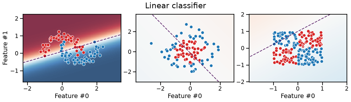
This confirms that it is not possible to separate the two classes with a linear model. On each plot we see a significant number of misclassified samples on the training set! The three plots show typical cases of underfitting for linear models.

Also, the last two plots show soft colors, meaning that the model is highly unsure about which class to choose.

Engineering non-linear features

As we did for the linear regression models, we now attempt to build a more expressive machine learning pipeline by leveraging non-linear feature engineering, with techniques such as binning, splines, polynomial features, and kernel approximation.

Let’s start with the binning transformation of the features:

from sklearn.preprocessing import KBinsDiscretizer

classifier = make_pipeline(
    KBinsDiscretizer(n_bins=5, encode="onehot"),  # already the default params
    LogisticRegression(),
)
classifier

Pipeline(steps=[('kbinsdiscretizer', KBinsDiscretizer()),
                ('logisticregression', LogisticRegression())])

In a Jupyter environment, please rerun this cell to show the HTML representation or trust the notebook.
On GitHub, the HTML representation is unable to render, please try loading this page with nbviewer.org.

plot_decision_boundary(classifier, title="Binning classifier")

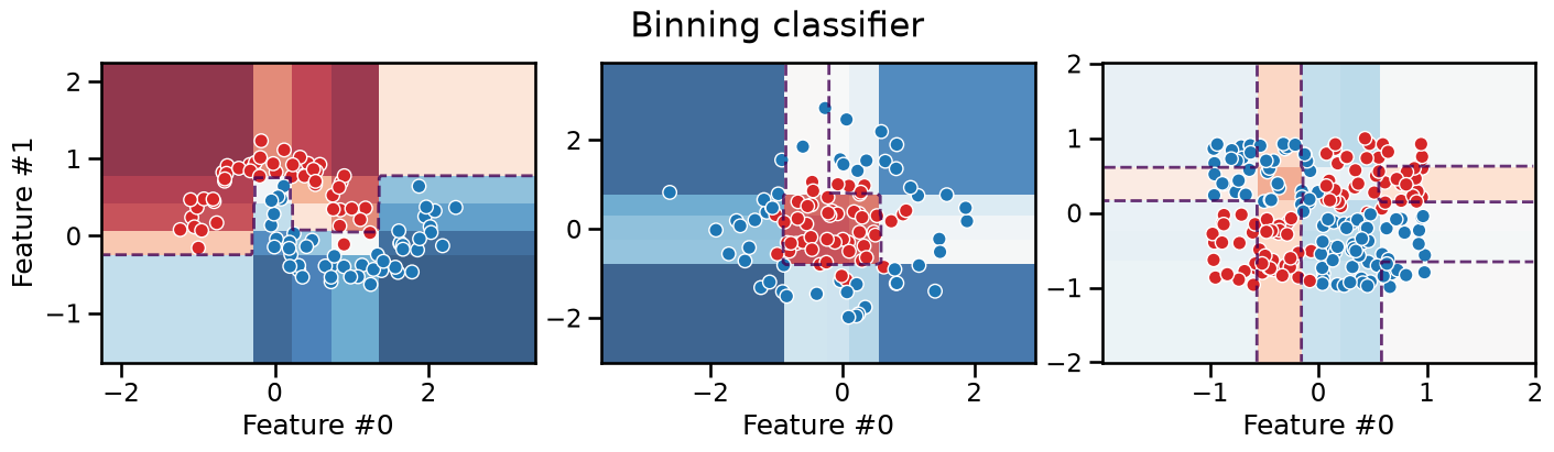
We can see that the resulting decision boundary is constrained to follow axis-aligned segments, which is very similar to what a decision tree would do as we will see in the next Module. Furthermore, as for decision trees, the model makes piecewise constant predictions within each rectangular region.

This axis-aligned decision boundary is not necessarily the natural decision boundary a human would have intuitively drawn for the moons dataset and the Gaussian quantiles datasets. It still makes it possible for the model to successfully separate the data. However, binning alone does not help the classifier separate the data for the XOR dataset. This is because the binning transformation is a feature-wise transformation and thus cannot capture interactions between features that are necessary to separate the XOR dataset.

Let’s now consider a spline transformation of the original features. This transformation can be considered a smooth version of the binning transformation. You can find more details in the scikit-learn user guide.

from sklearn.preprocessing import SplineTransformer

classifier = make_pipeline(
    SplineTransformer(degree=3, n_knots=5),
    LogisticRegression(),
)
classifier

Pipeline(steps=[('splinetransformer', SplineTransformer()),
                ('logisticregression', LogisticRegression())])

In a Jupyter environment, please rerun this cell to show the HTML representation or trust the notebook.
On GitHub, the HTML representation is unable to render, please try loading this page with nbviewer.org.

plot_decision_boundary(classifier, title="Spline classifier")

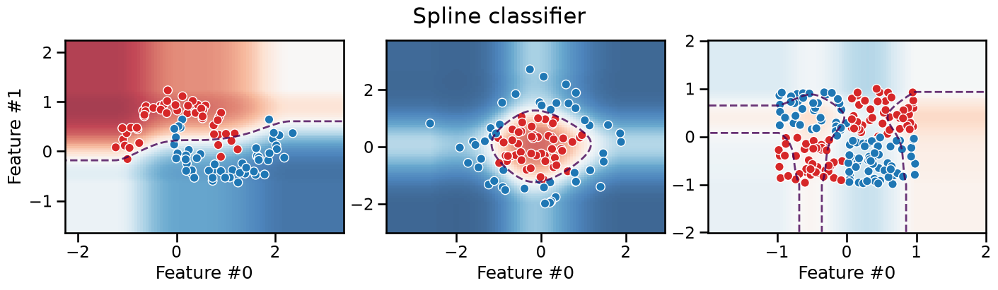
We can see that the decision boundary is now smooth, and while it favors axis-aligned decision rules when extrapolating in low density regions, it can adopt a more curvy decision boundary in the high density regions. However, as for the binning transformation, the model still fails to separate the data for the XOR dataset, irrespective of the number of knots, for the same reasons: the spline transformation is a feature-wise transformation and thus cannot capture interactions between features.

Take into account that the number of knots is a hyperparameter that needs to be tuned. If we use too few knots, the model would underfit the data, as shown on the moons dataset. If we use too many knots, the model would overfit the data.

Note

Notice that KBinsDiscretizer(encode="onehot") and SplineTransformer do not require additional scaling. Indeed, they can replace the scaling step for numerical features: they both create features with values in the [0, 1] range.

Modeling non-additive feature interactions

We now consider feature engineering techniques that non-linearly combine the original features in the hope of capturing interactions between them. We will consider polynomial features and kernel approximation.

Let’s start with the polynomial features:

from sklearn.preprocessing import PolynomialFeatures

classifier = make_pipeline(
    StandardScaler(),
    PolynomialFeatures(degree=3, include_bias=False),
    LogisticRegression(C=10),
)
classifier

Pipeline(steps=[('standardscaler', StandardScaler()),
                ('polynomialfeatures',
                 PolynomialFeatures(degree=3, include_bias=False)),
                ('logisticregression', LogisticRegression(C=10))])

In a Jupyter environment, please rerun this cell to show the HTML representation or trust the notebook.
On GitHub, the HTML representation is unable to render, please try loading this page with nbviewer.org.

plot_decision_boundary(classifier, title="Polynomial classifier")

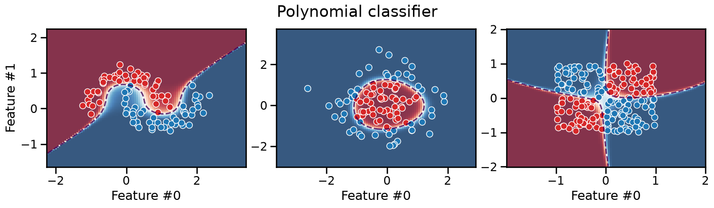
We can see that the decision boundary of this polynomial classifier is smooth and can successfully separate the data on all three datasets (depending on how we set the values of the degree and C hyperparameters).

It is interesting to observe that this models extrapolates very differently from the previous models: its decision boundary can take a diagonal direction. Furthermore, we can observe that predictions are very confident in the low density regions of the feature space, even very close to the decision boundary

We can obtain very similar results by using a kernel approximation technique such as the Nyström method with a polynomial kernel:

from sklearn.kernel_approximation import Nystroem

classifier = make_pipeline(
    StandardScaler(),
    Nystroem(kernel="poly", degree=3, coef0=1, n_components=100),
    LogisticRegression(C=10),
)
classifier

Pipeline(steps=[('standardscaler', StandardScaler()),
                ('nystroem', Nystroem(coef0=1, degree=3, kernel='poly')),
                ('logisticregression', LogisticRegression(C=10))])

In a Jupyter environment, please rerun this cell to show the HTML representation or trust the notebook.
On GitHub, the HTML representation is unable to render, please try loading this page with nbviewer.org.

plot_decision_boundary(classifier, title="Polynomial Nystroem classifier")

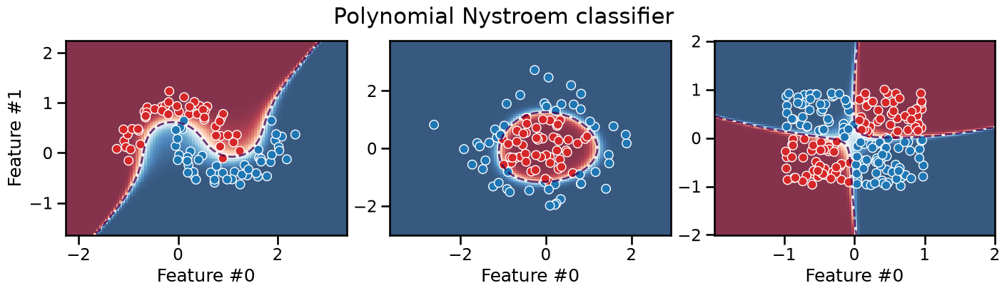
The polynomial kernel approach would be interesting in cases where the original feature space is already of high dimension: in these cases, computing the complete polynomial expansion with PolynomialFeatures could be intractable, while the Nyström method can control the output dimensionality with the n_components parameter.

Let’s now explore the use of a radial basis function (RBF) kernel:

from sklearn.kernel_approximation import Nystroem

classifier = make_pipeline(
    StandardScaler(),
    Nystroem(kernel="rbf", gamma=1, n_components=100),
    LogisticRegression(C=5),
)
classifier

Pipeline(steps=[('standardscaler', StandardScaler()),
                ('nystroem', Nystroem(gamma=1)),
                ('logisticregression', LogisticRegression(C=5))])

In a Jupyter environment, please rerun this cell to show the HTML representation or trust the notebook.
On GitHub, the HTML representation is unable to render, please try loading this page with nbviewer.org.

plot_decision_boundary(classifier, title="RBF Nystroem classifier")

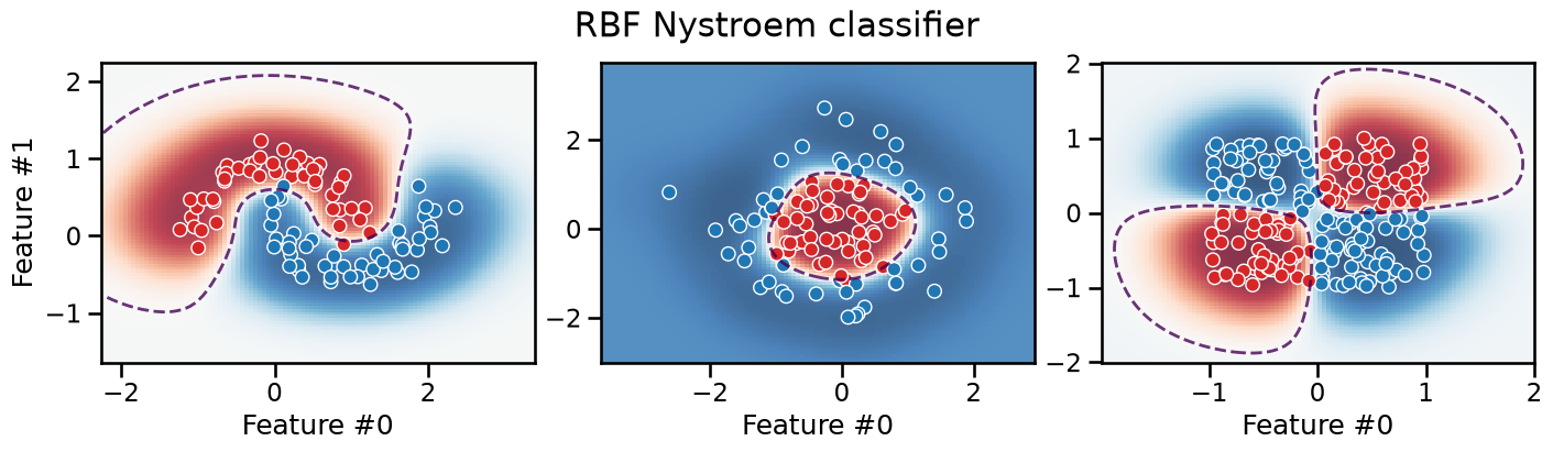
The resulting decision boundary is smooth and can successfully separate the classes for all three datasets. Furthemore, the model extrapolates very differently: in particular, it tends to be much less confident in its predictions in the low density regions of the feature space.

As for the previous polynomial pipelines, this pipeline does not favor axis-aligned decision rules. It can be shown mathematically that the inductive bias of our RBF pipeline is actually rotationally invariant.

Multi-step feature engineering

It is possible to combine several feature engineering transformers in a single pipeline to blend their respective inductive biases. For instance, we can combine the binning transformation with a kernel approximation:

classifier = make_pipeline(
    KBinsDiscretizer(n_bins=5),
    Nystroem(kernel="rbf", gamma=1.0, n_components=100),
    LogisticRegression(),
)
classifier

Pipeline(steps=[('kbinsdiscretizer', KBinsDiscretizer()),
                ('nystroem', Nystroem(gamma=1.0)),
                ('logisticregression', LogisticRegression())])

In a Jupyter environment, please rerun this cell to show the HTML representation or trust the notebook.
On GitHub, the HTML representation is unable to render, please try loading this page with nbviewer.org.

plot_decision_boundary(classifier, title="Binning + Nystroem classifier")

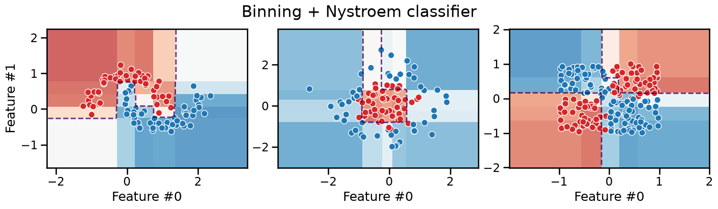
It is interesting to observe that this model is still piecewise constant with axis-aligned decision boundaries everywhere, but it can now successfully deal with the XOR problem thanks to the second step of the pipeline that can model the interactions between the features transformed by the first step.

We can also combine the spline transformation with a kernel approximation:

from sklearn.kernel_approximation import Nystroem

classifier = make_pipeline(
    SplineTransformer(n_knots=5),
    Nystroem(kernel="rbf", gamma=1.0, n_components=100),
    LogisticRegression(),
)
classifier

Pipeline(steps=[('splinetransformer', SplineTransformer()),
                ('nystroem', Nystroem(gamma=1.0)),
                ('logisticregression', LogisticRegression())])

In a Jupyter environment, please rerun this cell to show the HTML representation or trust the notebook.
On GitHub, the HTML representation is unable to render, please try loading this page with nbviewer.org.

plot_decision_boundary(classifier, title="Spline + RBF Nystroem classifier")

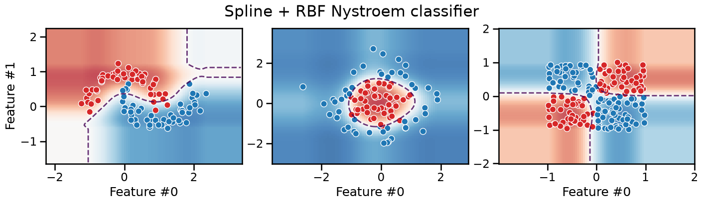
The decision boundary of this pipeline is smooth, but with axis-aligned extrapolation.

Depending on the task, this can be considered an advantage or a drawback.

Summary and take-away messages

• Linear models such as logistic regression can be used for classification on non-linearly separable datasets by leveraging non-linear feature engineering.

• Transformers such as KBinsDiscretizer and SplineTransformer can be used to engineer non-linear features independently for each original feature.

• As a result, these transformers cannot capture interactions between the orignal features (and then would fail on the XOR classification task).

• Despite this limitation they already augment the expressivity of the pipeline, which can be sufficient for some datasets.

• They also favor axis-aligned decision boundaries, in particular in the low density regions of the feature space (axis-aligned extrapolation).

• Transformers such as PolynomialFeatures and Nystroem can be used to engineer non-linear features that capture interactions between the original features.

• It can be useful to combine several feature engineering transformers in a single pipeline to build a more expressive model, for instance to favor axis-aligned extrapolation while also capturing interactions.

• In particular, if the original dataset has both numerical and categorical features, it can be useful to apply binning or a spline transformation to the numerical features and one-hot encoding to the categorical features. Then, the resulting features can be combined with a kernel approximation to model interactions between numerical and categorical features. This can be achieved with the help of ColumnTransformer.

In subsequent notebooks and exercises, we will further explore the interplay between regularization, feature engineering, and the under-fitting / overfitting trade-off.

But first we will do an exercise to illustrate the relationship between the Nyström kernel approximation and support vector machines.