📃 Solution for Exercise M4.02#
In a previous notebook we introduced the use of performance metrics to evaluate a clustering model when we have access to labeled data, namely the V-measure and Adjusted Rand Index (ARI). In this exercise you will get familiar with another supervised metric for clustering, known as Adjusted Mutual Information (AMI).
To illustrate the different concepts, we retain some of the features from the penguins dataset.
import pandas as pd

columns_to_keep = [
    "Culmen Length (mm)",
    "Culmen Depth (mm)",
    "Flipper Length (mm)",
    "Body Mass (g)",
    "Sex",
    "Species",
]
penguins = pd.read_csv("../datasets/penguins.csv")[columns_to_keep].dropna()
species = penguins["Species"].str.split(" ").str[0]
penguins = penguins.drop(columns=["Species"])
penguins
| Culmen Length (mm) | Culmen Depth (mm) | Flipper Length (mm) | Body Mass (g) | Sex | |
|---|---|---|---|---|---|
| 0 | 39.1 | 18.7 | 181.0 | 3750.0 | MALE |
| 1 | 39.5 | 17.4 | 186.0 | 3800.0 | FEMALE |
| 2 | 40.3 | 18.0 | 195.0 | 3250.0 | FEMALE |
| 4 | 36.7 | 19.3 | 193.0 | 3450.0 | FEMALE |
| 5 | 39.3 | 20.6 | 190.0 | 3650.0 | MALE |
| ... | ... | ... | ... | ... | ... |
| 339 | 55.8 | 19.8 | 207.0 | 4000.0 | MALE |
| 340 | 43.5 | 18.1 | 202.0 | 3400.0 | FEMALE |
| 341 | 49.6 | 18.2 | 193.0 | 3775.0 | MALE |
| 342 | 50.8 | 19.0 | 210.0 | 4100.0 | MALE |
| 343 | 50.2 | 18.7 | 198.0 | 3775.0 | FEMALE |
334 rows × 5 columns
We recall that the silhouette score presented a maximum when n_clusters=6
when using all of the features above (not the species). Our hypothesis was
that those clusters correspond to the 3 species of penguins present in the
dataset (Adelie, Chinstrap, and Gentoo) further splitted by Sex (2 clusters
for each species).
Repeat the same pipeline consisting of a OneHotEncoder with
drop="if_binary" for the “Sex” column, a StandardScaler for the other
columns. The final estimator should be KMeans with n_clusters=6. You can
set the random_state for reproducibility, but that should not change the
interpretation of the results.
# solution
from sklearn.compose import make_column_transformer, make_column_selector
from sklearn.pipeline import make_pipeline
from sklearn.preprocessing import StandardScaler, OneHotEncoder
from sklearn.cluster import KMeans

preprocessor = make_column_transformer(
    (
        OneHotEncoder(drop="if_binary"),
        make_column_selector(dtype_exclude="number"),
    ),
    (
        StandardScaler(),
        make_column_selector(dtype_include="number"),
    ),
)

model = make_pipeline(
    preprocessor,
    KMeans(n_clusters=6, random_state=0),
)
Make two sns.scatterplot of “Culmen Length (mm)” versus “Flipper Length
(mm)”, side-by-side. On one of them, the hue should be the “species and sex”
coming from the known information in the dataset, and the hue in the other
should be the cluster labels.
Only the colors may differ, as the ordering of the labels is arbitrary (both for the k-means cluster and the “true” labels).
# solution
import matplotlib.pyplot as plt
import seaborn as sns

species_and_sex_labels = species + " " + penguins["Sex"]
cluster_labels = model.fit_predict(penguins)

fig, (ax1, ax2) = plt.subplots(1, 2, sharey=True, figsize=(14, 7))
sns.scatterplot(
    penguins.assign(species_and_sex=species_and_sex_labels),
    hue="species_and_sex",
    x="Culmen Length (mm)",
    y="Flipper Length (mm)",
    palette="deep",
    alpha=0.7,
    ax=ax1,
    legend=None,
)
ax1.set_title("Species and sex")
sns.scatterplot(
    penguins.assign(kmeans_labels=cluster_labels),
    hue="kmeans_labels",
    x="Culmen Length (mm)",
    y="Flipper Length (mm)",
    palette="deep",
    alpha=0.7,
    ax=ax2,
    legend=None,
)
_ = ax2.set_title("K-means labels")
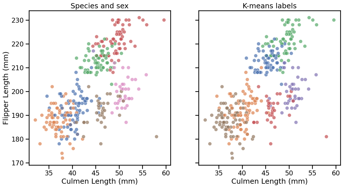
We now have a visual intuition of the agreement between the clusters found by k-means and the combination of the “Species” and “Sex” labels. We can further quantify it using the Adjusted Mutual Information (AMI) score.
Use
sklearn.metrics.adjusted_mutual_info_score
to compare both sets of labels. The AMI returns a value of 1 when the two
partitions are identical (ie perfectly matched)
# solution
from sklearn.metrics import adjusted_mutual_info_score

ami = adjusted_mutual_info_score(
    species_and_sex_labels,
    cluster_labels,
)
print(f"Adjusted Mutual Information (AMI): {ami:.3f}")
Adjusted Mutual Information (AMI): 0.957
This value is very close to 1.0, which indicates a very strong agreement. This confirms our visual intuition that the 6 clusters found by k-means nearly exactly correspond to the species crossed with the sex of the penguins.
Now use a
sklearn.preprocessing.LabelEncoder
to fit_transform the “true” labels (coming from combinations of species and
sex). What would be the accuracy if we tried to use it to measure the
agreement between both sets of labels?
# solution
from sklearn.preprocessing import LabelEncoder
from sklearn.metrics import accuracy_score

true_labels = LabelEncoder().fit_transform(species_and_sex_labels)

cluster_labels = model.fit_predict(penguins)
acc = accuracy_score(true_labels, cluster_labels)
print(f"Accuracy: {acc:.3f}")
Accuracy: 0.213
The accuracy is misleadingly low. It is not a valid metric for clustering unless you map labels explicitly.
Permute the cluster labels using np.random.permutation, then compute both
the AMI and the accuracy when comparing the true and permuted labels. Are they
sensitive to relabeling?
# solution
import numpy as np

rng = np.random.RandomState(0)
unique_labels = np.unique(cluster_labels)
permutation = rng.permutation(unique_labels)
permuted_labels = np.zeros_like(cluster_labels)

for original, new in zip(unique_labels, permutation):
    permuted_labels[cluster_labels == original] = new

permuted_ami = adjusted_mutual_info_score(true_labels, permuted_labels)
permuted_acc = accuracy_score(true_labels, permuted_labels)

print(f"AMI (permuted): {permuted_ami:.3f}")
print(f"Accuracy (permuted): {permuted_acc:.3f}")
AMI (permuted): 0.957
Accuracy (permuted): 0.174
AMI stays the same because the cluster structure has not changed, only the labels’ names: AMI is invariant to a random permutation of the labels.
The accuracy changes because it is only meaningful when the ordering of the clustering labels have been mapped correctly to ordering the human labels which has very little chance of happening when randomly permuting the labels.
AMI is designed to return a value near zero (it can be negative) when the clustering is no better than random.
To understand how AMI corrects for chance, compare the true labels with a
completely random labeling using np.random.randint to generate as many
labels as rows in the dataset, each containing a value between 0 and 5 (to
match the number of clusters).
# solution
for _ in range(10):
    random_labels = rng.randint(0, len(unique_labels), size=len(species))
    ami_random = adjusted_mutual_info_score(true_labels, random_labels)
    print(f"AMI (random labels): {ami_random:.3f}")
AMI (random labels): 0.001
AMI (random labels): -0.007
AMI (random labels): 0.014
AMI (random labels): -0.012
AMI (random labels): -0.008
AMI (random labels): -0.001
AMI (random labels): -0.007
AMI (random labels): -0.009
AMI (random labels): -0.005
AMI (random labels): 0.015
We observe either positive or negative values but always very close to zero depending the particular random labels generated.
We can conclude by comparing AMI to other metrics:
Adjusted Rand Index (ARI): Also corrects for chance, but it counts pairs of points, in other words, how many pairs that are together in the true labels are also together in the clusters. It is combinatorial, not based on information-theory as AMI.
V-measure: Based on homogeneity (do clusters contain mostly one class?) and completeness (are all members of a class grouped together?), but it does not correct for chance. If you run a random clustering, V-measure might still give a misleadingly non-zero score, unlike AMI or ARI.